Technical note: Improving the AWAT filter with interpolation schemes for advanced processing of high resolution data

www.hydrol-earth-syst-sci.net/20/2309/2016/ doi:10.5194/hess-20-2309-2016

© Author(s) 2016. CC Attribution 3.0 License.

Technical note: Improving the AWAT filter with interpolation

schemes for advanced processing of high resolution data

Andre Peters, Thomas Nehls, and Gerd Wessolek

Institut für Ökologie, Technische Universität Berlin, Berlin, 10587, Germany

Correspondence to:Andre Peters ([email protected])

Received: 29 January 2016 – Published in Hydrol. Earth Syst. Sci. Discuss.: 21 March 2016 Revised: 20 May 2016 – Accepted: 20 May 2016 – Published: 15 June 2016

Abstract. Weighing lysimeters with appropriate data filter-ing yield the most precise and unbiased information for pre-cipitation (P) and evapotranspiration (ET). A recently intro-duced filter scheme for such data is the AWAT (Adaptive Window and Adaptive Threshold) filter (Peters et al., 2014). The filter applies an adaptive threshold to separate significant from insignificant mass changes, guaranteeing thatP and ET are not overestimated, and uses a step interpolation between the significant mass changes. In this contribution we show that the step interpolation scheme, which reflects the reso-lution of the measuring system, can lead to unrealistic pre-diction ofP and ET, especially if they are required in high temporal resolution. We introduce linear and spline interpo-lation schemes to overcome these problems. To guarantee that medium to strong precipitation events abruptly following low or zero fluxes are not smoothed in an unfavourable way, a simple heuristic selection criterion is used, which attributes such precipitations to the step interpolation. The three inter-polation schemes (step, linear and spline) are tested and com-pared using a data set from a grass-reference lysimeter with 1 min resolution, ranging from 1 January to 5 August 2014. The selected output resolutions forP and ET prediction are 1 day, 1 h and 10 min. As expected, the step scheme yielded reasonable flux rates only for a resolution of 1 day, whereas the other two schemes are well able to yield reasonable re-sults for any resolution. The spline scheme returned slightly better results than the linear scheme concerning the differ-ences between filtered values and raw data. Moreover, this scheme allows continuous differentiability of filtered data so that any output resolution for the fluxes is sound. Since com-putational burden is not problematic for any of the interpola-tion schemes, we suggest always using the spline scheme.

1 Introduction

Precipitation (P (L T−1)) and evapotranspiration (ET (L T−1)) have to be precisely known to answer many ques-tions regarding water, solute and energy fluxes in the soil– plant atmosphere continuum. In several simulation studies, the precise values forP and ET are required only as daily averages (e.g. Schelle et al., 2012). However, in other cases the diurnal course ofP and ET must be known, e.g. whether root water uptake shall be simulated with a physically based model (Javaux et al., 2008; Couvreur et al., 2012) or macro-pore flow due to heavy but short precipitation events be sim-ulated under realistic conditions (Malone et al., 2004; Mc-Grath et al., 2008).

Today, weighing lysimeter measurements with a high mass and temporal resolution yield the most precise values for both P and ET. This is since systematic as well as random er-rors are largely eliminated, the former due to their installa-tion height exactly at ground surface and the latter due to the relatively large size in comparison to other devices. The high temporal resolution of the measurement is required to dis-tinguish betweenP and ET, which might follow each other even in small time intervals.

in system mass is interpreted as precipitation and each de-crease as evapotranspiration.

As already suggested by Fank (2013) and Schrader et al. (2013), such filter routines can be carried out in two steps. First a smoothing routine (for example a simple moving av-erage) with a certain window widthw(T) is applied and sec-ond all changes of the smoothed data smaller than a prede-fined threshold valueδ(L) are discarded. The second step is mandatory to avoid small changes in the smoothed data be-ing interpreted asP and ET. Schrader et al. (2013) showed that there are no “ideal” values for w or δ within a longer time interval because at some events small values forwand δ are required, whereas at other events high values forwor δare required to get the maximum information content from the data.

Therefore, Peters et al. (2014) suggested the so-called AWAT (Adaptive Window Adaptive Threshold) filter. The in-novation in the AWAT filter consists in the variability ofw andδ, which are adjusted according to the characteristics of the measured data. If the signal strength is high (e.g. due to precipitation),wgets small, and if signal strength is low,w gets large. Similarly, if noise is high,δgets large, and if it is low,δ gets small. The AWAT filter was successfully applied in recent studies (Gebler, et al., 2015; Hannes et al., 2015; Hoffmann et al., 2016).

The threshold approach makes sure that significant weight changes are separated from insignificant changes and leads to a step-like course of the calculated cumulative upper bound-ary flux (see Fig. 6 in Schrader et al., 2013, or Figs. 6 and 7 in Peters et al., 2014). The points in time at which the steps oc-cur can be called anchor points and all other points are mere interpolated data.

ET andP are given as the first derivatives of the cumula-tive upper boundary flux and are commonly required as the mean for an application-specific time interval. Since the time span between two anchor points is usually much smaller than 1 day, the step interpolation scheme gives fairly good results if only daily resolution is required. However, if the required time interval for the upper boundary flux is much smaller than the time span between the anchor points (e.g. 1 h or even 10 min), the step interpolation yields unrealistic values: at time intervals between two subsequent anchor points the cal-culated flux is zero. If a time interval comprises one anchor point, the calculated flux is large. Moreover, the magnitude of the flux depends on the length of the chosen time inter-val since the step occurs immediately. Using such data will probably lead to erroneous simulations and also to numerical problems due to abrupt changes in the boundary conditions, with high fluxes alternating with no fluxes.

Note that the step scheme with the abrupt changes directly reflects the resolution of the system. If no further assump-tions about the underlying process are justified, this is the maximum information which can be derived from the mea-suring set-up. However, many flux processes at the interface between the soil–plant system and the atmosphere, such as

ET or dew fall, are known to be rather smooth and continu-ous than abrupt.

The aim of this contribution is (i) to show the impact of the step interpolation scheme on calculated fluxes for different time intervals and (ii) to improve the AWAT filter by elim-inating the above mentioned problems using linear or cubic Hermitian spline interpolation schemes between the anchor points. This leads to a smoothing of the steps but guarantees that the cumulated fluxes are still exactly the same as in the original approach.

2 Material and methods 2.1 Lysimeter set-up

The measurements were conducted at the Berlin-Marienfelde (52.396731◦N, 13.367524◦E) lysimeter station. The lysime-ter was a so-called grass-reference lysimelysime-ter with simulated groundwater depth at 1.3 m. It was 1.5 m deep with a sur-face area of 1 m2. A lever-arm counterbalance system was combined with a laboratory scale, which resulted in an over-all resolution of the system of 100 g, which corresponds to approximately 0.1 mm for the upper boundary fluxes. The outflow/inflow of water at the lower boundary was directly recorded with a scale with a resolution of 5 g. The data were logged in a 1 min time interval.

The soil material was a packed silt loam taken from a Haplic Phaeozem, which ensures good capillary connection between groundwater level and the root system. The 20 cm bottom layer consisted of fully water saturated gravel. The 12 cm high grass on the lysimeters was a mixture ofLolium perenne,Festuca arundinaceaandPoa pratensis, three cool-season grass species with large rooting depths.

2.2 Data processing

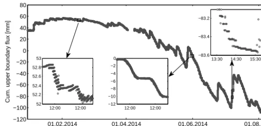
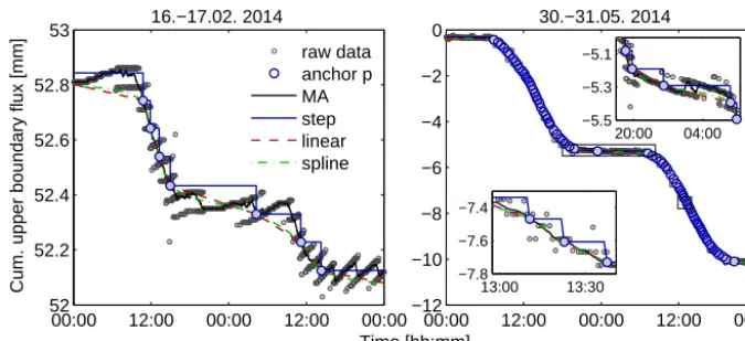
The data for this study were recorded from 1 January to 5 August 2014 (Fig. 1). Between 2 and 8 April no data were available due to malfunction of the lysimeter scale. In order to evaluate the interpolation schemes, we focussed on three time intervals: (i) 16–17 February 2014, representing very low evaporation rates, (ii) 30–31 Mai 2014, representing high evaporation rates, and (iii) 7 July 2014 between 13:30 and 15:30, representing the start of a heavy rainfall event.

01.02.2014 01.04.2014 01.06.2014 01.08.2014 −120

−100 −80 −60 −40 −20 0 20 40 60 80

Date

Cum. upper boundary flux [mm]

12:00 12:00 52

52.2 52.4 52.6 52.8 53

12:00 12:00 −12

−10 −8 −6 −4 −2

0 −83.613:30 14:30 15:30

−83.4 −83.2

Figure 1.Raw data for the cumulative upper boundary flux of a grass covered lysimeter in Berlin-Marienfelde, Germany. The data of the three selected time intervals on 16–17 February 2014, 30–31 May 2014, and 7 July 2014 between 13:30 and 15:30 are given in the three subplots. Note that the time and flux intervals for the three intervals are different in the subplots.

2.3 Threshold and interpolation schemes

The complete filter scheme is given in detail in Peters et al. (2014) and is therefore not explained here. The filter was applied using a minimum window width of 1 min, a maxi-mum window width of 31 min, a minimaxi-mum threshold value of 0.1 mm, and a maximum threshold value of 0.24 mm. 2.3.1 Step interpolation scheme

After the moving average (MA) is calculated, the thresh-old routine distinguishes between significant and insignifi-cant mass changes starting with the first value of the MA at t=0, which might be called the first anchor point ap0. This

value is kept for all subsequent time steps until the difference between the corresponding value of the MA and the anchor point ap0is greater than the threshold valueδ. Then, the new

value is the next anchor point ap1(see Fig. 2 for illustration).

This leads to a stepwise course of the calculated cumulative upper boundary flux.

All values between the anchor points can be regarded as interpolated values, whereas the anchor points coincide ex-actly with the MA. This procedure guarantees that small os-cillations, which occur even after smoothing the data, will not be regarded as real mass changes and thus interpreted as evapotranspiration or precipitation.

2.3.2 Linear and spline interpolation schemes

In order to prevent the problems discussed above, which arise from the step scheme for the upper boundary flux, alternative interpolation schemes can be used. The simplest way is to calculate a linear interpolation between two subsequent an-chor points. An alternative is the use of piecewise Hermi-tian splines (Fritsch and Carlson, 1980), which smooth the time course of the upper flux but do not oscillate like sim-ple splines. Cubic Hermitian splines are frequently used in soil hydrology, e.g. for the description of hydraulic functions (Iden and Durner, 2007) or for temporal interpolation of

mea-sured values in evaporation experiments (Peters and Durner, 2008; Peters et al., 2015). In contrast to the linear interpola-tion scheme, the spline interpolainterpola-tion yields a smooth curve at the anchor points and is thus even continuously differen-tiable.

00:00 12:00 00:00 12:00 00:00 −12

−10 −8 −6 −4 −2

0 30.−31.05. 2014

20:00 04:00

−5.5 −5.3 −5.1

13:00 13:30

−7.8 −7.6 −7.4

00:00 12:00 00:00 12:00 00:00

52 52.2 52.4 52.6 52.8 53

Time [hh:mm]

Cum. upper boundary flux [mm]

16.−17.02. 2014

raw data anchor p MA step linear spline

Figure 2.Raw data of two evapotranspiration events, filtered with the original AWAT filter (steps) and linear as well as spline interpolation schemes. Left: low evapotranspiration on 16–17 February 2014; right: high evapotranspiration rates on 30–31 May 2014.

The linear interpolation scheme as well as the cubic Her-mitian spline interpolation routine of Fritsch and Carlson (1980) were implemented in the AWAT code (Peters et al., 2014). In this study all three interpolation schemes (steps, linear, splines) witha=1.1 for the linear and spline interpo-lations are applied and compared. In order to test the impor-tance of the rain correction, we additionally applied the linear and spline interpolation schemes without rain correction, set-tingato the very high value of 9999 (linear∗, spline∗). This guaranteed that the criterion1M > aδis never met.

The fluxes were calculated for time intervals of 1 day, 1 h, and 10 min. The calculated evapotranspiration rates for the three different schemes and time intervals were then com-pared for the two time spans at 16–17 February 2014 and 30–31 May 2014. The performance of the different schemes, including linear∗ and spline∗, with respect to precipitation following a time with low fluxes was compared for the time span on 7 July 2014 between 13:30 and 15:30. Finally, the biases of the different schemes were compared for the com-plete data set by analysing the residuals between filtered and measured data.

2.3.3 Definition of bias term

The time series of observations (O) can be decomposed as signal and noise:

O=R+N, (1)

where R are the unknown real values andN is the noise. Then the filtered and interpolated time seriesF (as described above) is given by

FMA(O)=FMA(R+N ), (2)

where MA is the moving average time series. By definition the bias ofF (bF) is

bF :=E

F (MA)−E(R), (3)

whereE is the linear expected value operator. Considering Eq. (1) yields

bF =E

F (MA)

−E(O)−E(N ). (4)

Note that the bias of the first filter step (MA) is given by

bMA=E(MA)−E(O)−E(N ), (5)

if we assume E(N )=0 andE(MA)−E(O)=0 leads to bMA=0 and

bF =E

F (MA)−E(O). (6)

E(N )=0 means that wind and other disturbing factors do not have any significant systematic effects, and E(MA)− E(O)=0 means that the MA does not lead to systematic de-viations between smoothed data and observations. The latter is only given for (i) very small signals, i.e. if the real val-ues (R) in the time windowware very similar, or (ii) ifw is small, which is the case for the AWAT filter when signals are strong. Thus these assumptions are reasonable and allow one to use the distribution of residuals between the mere MA and raw data as a reference for the distribution of residuals between interpolated data and raw data.

3 Results

Time [hh:mm] 00:000 12:00 00:00 12:00 00:00

1 2 3

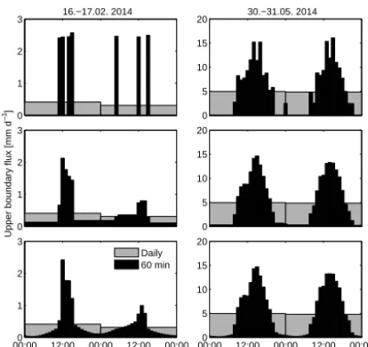
Daily 60 min

00:000 12:00 00:00 12:00 00:00 5

10 15 20

Spline

0 1 2 3

Upper boundary flux [mm d ] 0 5 10 15 20

Linear

0 1 2

3 16.−17.02. 2014

0 5 10 15 20

Steps

30.−31.05. 2014

–1

Figure 3. Derived potential evapotranspiration rates from data shown in Fig. 2 with temporal resolutions of 1 day or 1 h, re-spectively. Steps: original step interpolation scheme; linear: linear interpolation scheme; spline: cubic Hermitian spline interpolation scheme.

original routine leads to larger differences between inter-polated and MA smoothed values. The differences increase with increasing time between two anchor points and with creasing time from the last anchor point. Moreover, this in-terpolation scheme leads to single, very high changes at the steps and no fluxes during the other time periods, which is especially problematic at low evapotranspiration rates, e.g. at night (see the step in the upper subplot in Fig. 2, right) or in winter (Fig. 2, left), where the continuously low ET fluxes of several hours are lumped into one single step.

Both the linear and spline interpolations lead to smoothed cumulative fluxes, closer to the MA values (Fig. 2). The dif-ferences between linear and spline interpolated cumulative fluxes are negligible except that the spline interpolation leads to slightly more smoothing. The different schemes will have an influence on calculated fluxes for small time intervals, as will be shown next.

3.2 Effect on calculated fluxes with different temporal resolution

3.2.1 One-day versus one-hour intervals

If the required temporal resolution is only 1 day, the orig-inal AWAT filter routine with step interpolation yields suf-ficient results, since the time intervals between two anchor points are much smaller than 1 day. The resulting evapotran-spiration rates are shown as grey bars in Fig. 3. However, if the required resolution is 1 h, the original step interpola-tion scheme yields very unrealistic fluxes, especially if po-tential ET is low (e.g. during night time, or in winter). If a

Time [hh:mm] 00:000 12:00 00:00 12:00 00:00

1 2 3

Daily 10 min

00:000 12:00 00:00 12:00 00:00 5

10 15 20

Spline

0 1 2 3

Upper boundary flux [mm d ] 0 5 10 15 20

Linear

0 5 10 15

20 16.−17.02. 2014

0 10 20 30 40

Steps

30.−31.05. 2014

–1

Figure 4. Derived potential evapotranspiration rates from data shown in Fig. 2 with temporal resolutions of 1 day or 10 min, re-spectively. Steps: original step interpolation scheme; linear: linear interpolation scheme; spline: cubic Hermitian spline interpolation scheme. Note different scales on ordinates for the step scheme be-tween Figs. 4 and 3.

step occurs within an interval, the calculated flux is high, otherwise the flux is zero (Fig. 3, top). The calculated ET reaches a maximum of 15 mm d−1in May and approximately 2.5 mm d−1in February.

The linear (Fig. 3, centre) or spline (Fig. 3, bottom) in-terpolation schemes lead to smooth and more realistic evap-otranspiration prediction. During day time both schemes yield comparable results. However, during night time, the linear scheme predicts small constant ET between two an-chor points, whereas the spline scheme predicts a decreasing course until the inflection point between two anchor points is reached, followed by increasing ET again.

3.2.2 Ten-minute intervals

Figure 5. Relative residual frequency distribution for the complete data set and the different interpolation schemes. Blue bars indicate residuals between original and filtered data for the cases with mere smoothing, omitting the threshold values; red bars indicate cases with

threshold values and subsequent interpolation. The broad bars at plot edges comprise all residuals greater than 0.25 or smaller than−0.25 mm.

Steps: original step interpolation scheme; linear: linear interpolation scheme; spline: cubic Hermitian spline interpolation scheme.

with very high fluxes in very short time intervals, selecting such small intervals is important for many simulation studies regarding a realistic expression of precipitation. Only with the new interpolation schemes can such precipitation events be described in combination with evapotranspiration events within the same temporal resolution.

3.3 Analysing residuals

Figure 5 shows the frequency distribution of the residuals between filtered and measured data. The blue bars show the residuals for the case without a threshold value, i.e. for the sole MA, and are thus the same for all three compared schemes. These residuals are symmetrically distributed with a zero mean, which is expected from a moving average with relatively small window widths, ranging from 1 to 31 min. Thus, if the raw data are regarded as being unbiased, the MA can also be regarded as unbiased.

Applying the original step interpolation scheme (Fig. 5, left, red bars) yields a bias towards negative values with a mean of−0.035 mm. This tendency towards negative values is explained by the fact that this interpolation scheme sticks to the mass values at the old anchor points until the thresh-old is reached, leading to overestimations of precipitation and underestimations of evapotranspiration periods, with the lat-ter exceeding the former (Pelat-ters et al., 2014). Note that ap-plying filters with fixed wandδ yields even greater biases (see Fig. 8 in Peters et al., 2014).

The simple linear interpolation scheme (Fig. 5, centre) leads to a more than three-fold smaller bias of 0.01 mm, with a slight tendency towards positive values. The spline scheme (right) even leads to a slightly smaller deviation. Thus, the linear and spline interpolation schemes are not only superior for the selected time spans in February and May, but also for the complete measured period. The additional computational burden is only minor for any interpolation scheme in com-parison with the preceding AWAT filtering. Thus, we suggest always using the spline scheme.

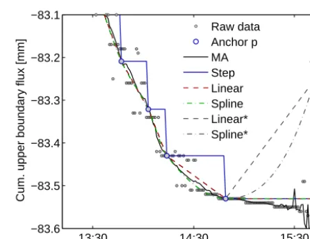
13:30 14:30 15:30

−83.6 −83.5 −83.4 −83.3 −83.2 −83.1

Time [hh:mm]

Cum. upper boundary flux [mm]

Raw data Anchor p MA Step Linear Spline Linear* Spline*

Figure 6.Raw data of a period of evapotranspiration followed by a precipitation event on 7 July 2014. Anchor p: anchor point; MA: moving average; steps: original step interpolation scheme; linear: linear interpolation scheme; spline: cubic Hermitian spline

inter-polation scheme; linear∗: linear interpolation scheme without

pre-cipitation correction; spline∗: cubic Hermitian spline interpolation

scheme without precipitation correction.

3.4 Effect on rain events

If a relatively strong precipitation event follows a pro-longed period with no significant flux, the mere interpola-tion schemes without rain correcinterpola-tion smooth such an event in an unrealistic manner (linear∗and spline∗in Fig. 6). The heuristic selection criterion determines that the step interpo-lation is kept for time intervals between two anchor points if 1M >1.1δ (linear and spline). This prevents unfavourable smoothing at the beginning of rain events.

4 Summary and conclusions

changes for short time intervals. This is most pronounced when real fluxes are small and therefore the distance between two anchor points is similar to or larger than the chosen time interval. This is problematic if highly resolved boundary con-ditions are needed for e.g. physically based simulations of water and energy fluxes in the soil–plant atmosphere system. Improving the filter by the proposed interpolation schemes solves this problem, leading to smoothed values, which are more realistic, especially for evapotranspiration events. Moreover, the spline scheme allows even a continuous differ-entiation and thus any temporal resolution for the predicted fluxes. A simple heuristic selection criterion, which sepa-rates medium to strong precipitation from all other events, prevents such precipitations from being smoothed in an un-favourable way. Thus, upper boundary conditions for phys-ically based simulations with very short time intervals can now be automatically derived from precision lysimeters.

In this study, we used a counterbalance weighing system with approximately 0.1 mm resolution. Modern lysimeters resting on weighing cells (von Unold and Fank, 2008) can have a resolution of up to 0.01 mm. Then, the problems of the step interpolation scheme are less pronounced but still present, specifically at times with low fluxes. Thus, the pro-posed solution is important, especially for lysimeters with limited resolution, which are still often used, but is also favourable for systems with higher resolution.

Note that the results and conclusions regarding the interpo-lation schemes hold also for filters with fixed window widths and threshold values (e.g. Fank, 2013; Schrader et al., 2013).

Acknowledgements. This study was financially supported by the Deutsche Forschungsgemeinschaft (DFG grant PE 1912/2-1). We thank Michael Facklam, Reinhild Schwartengräber, Björn Kluge, Joachim Buchholz and Steffen Trinks for their assis-tance with the lysimeter construction and maintenance. We also thank Marnik Vanclooster as Associate Editor and Johann Fank, Thomas Pütz and one anonymous reviewer for their insightful comments and suggestions, which greatly improved the manuscript.

Edited by: M. Vanclooster

References

Couvreur, V., Vanderborght, J., and Javaux, M.: A simple three-dimensional macroscopic root water uptake model based on the hydraulic architecture approach, Hydrol. Earth Syst. Sci., 16, 2957–2971, doi:10.5194/hess-16-2957-2012, 2012.

Fank, J.: Wasserbilanzauswertung aus Präzisionslysimeterdaten, in: 15. Gumpensteiner Lysimetertagung 2013, Lehr- und Forschungszentrum für Landwirtschaft Raumberg-Gumpenstein, Irdning, Austria, 85–92, 2013.

Fritsch, F. N. and Carlson R. E.: Monotone piecewise cubic inter-polation, SIAM J. Numer. Anal., 17, 238–246, 1980.

Gebler, S., Hendricks Franssen, H.-J., Pütz, T., Post, H., Schmidt, M., and Vereecken, H.: Actual evapotranspiration and precipi-tation measured by lysimeters: a comparison with eddy

covari-ance and tipping bucket, Hydrol. Earth Syst. Sci., 19, 2145–2161, doi:10.5194/hess-19-2145-2015, 2015.

Hannes, M., Wollschläger, U., Schrader, F., Durner, W., Gebler, S., Pütz, T., Fank, J., von Unold, G., and Vogel, H.-J.: A compre-hensive filtering scheme for high-resolution estimation of the water balance components from high-precision lysimeters, Hy-drol. Earth Syst. Sci., 19, 3405–3418, doi:10.5194/hess-19-3405-2015, 2015.

Hoffmann, M., Schwartengräber, R., Wessolek, G., and Peters, A.: Comparison of simple rain gauge measurements with precision lysimeter data, Atmos. Res., 174–175, 120–123, 2016.

Iden, S. C. and Durner, W.: Free-form estimation of the un-saturated soil hydraulic properties by inverse modeling us-ing global optimization, Water Resour. Res., 43, W07451, doi:10.1029/2006WR005845, 2007.

Javaux, M., Schröder, T., Vanderborght, J., and Vereecken, H.: Use of a three-dimensional detailed modelling approach for predict-ing root water uptake, Vadose Zone J., 7, 1079–1088, 2008. Malone, R. W., Weatherington-Rice, J., Shipitalo, M. J., Fausey, N.,

Ma, L., Ahuja, L. R., Don Wauchope, R., and Ma, Q.: Herbicide leaching as affected by macropore flow and within-storm rainfall intensity variation: A RZWQM simulation, Pest Manag. Sci., 60, 277–285, 2004.

McGrath, G. S., Hinz, C., and Sivapalan, M.: Modelling the impact of within-storm variability of rainfall on the loading of solutes to preferential flow pathways, Eur. J. Soil Sci., 59, 24–33, 2008. Meissner, R., Seeger, J., Rupp, H., Seyfarth, M., and Borg, H.:

Measurement of dew, fog, and rime with a high-precision gravitation lysimeter, J. Plant Nutr. Soil Sc., 170, 335–344, doi:10.1002/jpln.200625002, 2007.

Nolz, R., Kammerer, G., and Cepuder, P.: Interpretation of lysimeter weighing data affected by wind, J. Plant Nutr. Soil Sc., 176, 200– 208, doi:10.1002/jpln.201200342, 2013.

Peters, A. and Durner, W.: Simplified evaporation method for de-termining soil hydraulic properties, J. Hydrol., 356, 147–162, doi:10.1016/j.jhydrol.2008.04.016, 2008.

Peters, A., Nehls, T., Schonsky, H., and Wessolek, G.: Separating precipitation and evapotranspiration from noise – a new filter routine for high-resolution lysimeter data, Hydrol. Earth Syst. Sci., 18, 1189–1198, doi:10.5194/hess-18-1189-2014, 2014. Peters, A. Iden, S. C., and Durner, W.: Revisiting the simplified

evaporation method: Identification of hydraulic functions con-sidering vapor, film and corner flow, J. Hydrol., 527, 531–542, doi:10.1016/j.jhydrol.2015.05.020, 2015.

Schelle, H., Iden, S. C., Fank, J., and Durner, W.: Inverse Estima-tion of Soil Hydraulic and Root DistribuEstima-tion Parameters from Lysimeter Data, Vadose Zone J., 11, doi:10.2136/vzj2011.0169, 2012.

Schrader, F., Durner, W., Fank, J., Gebler, S., Pütz, T., Hannes, M., and Wollschläger, U.: Estimating precipitation and actual evapotranspiration from precision lysimeter measurements, in: Four Decades of Progress in Monitoring and Modeling of Pro-cesses in the Soil-Plant-Atmosphere System: Applications and Challenges, edited by: Romano, N., D’Urso, G., Severino, G., Chirico, G., and Palladino, M., Procedia Environmental Sci-ences, 543–552, 2013.