Large scale hydrological modelling by using modified PUB recommendations: the India HYPE case

www.hydrol-earth-syst-sci.net/19/4559/2015/ doi:10.5194/hess-19-4559-2015

© Author(s) 2015. CC Attribution 3.0 License.

Large-scale hydrological modelling by using modified PUB

recommendations: the India-HYPE case

I. G. Pechlivanidis and B. Arheimer

Swedish Meteorological and Hydrological Institute, Norrköping, Sweden Correspondence to: I. G. Pechlivanidis ([email protected])

Received: 13 February 2015 – Published in Hydrol. Earth Syst. Sci. Discuss.: 10 March 2015 Revised: 23 October 2015 – Accepted: 26 October 2015 – Published: 17 November 2015

Abstract. The scientific initiative Prediction in Ungauged Basins (PUB) (2003–2012 by the IAHS) put considerable ef-fort into improving the reliability of hydrological models to predict flow response in ungauged rivers. PUB’s collective experience advanced hydrologic science and defined guide-lines to make predictions in catchments without observed runoff data. At present, there is a raised interest in applying catchment models to large domains and large data samples in a multi-basin manner, to explore emerging spatial patterns or learn from comparative hydrology. However, such mod-elling involves additional sources of uncertainties caused by the inconsistency between input data sets, i.e. particularly regional and global databases. This may lead to inaccurate model parameterisation and erroneous process understand-ing. In order to bridge the gap between the best practices for flow predictions in single catchments and multi-basins at the large scale, we present a further developed and slightly modified version of the recommended best practices for PUB by Takeuchi et al. (2013). By using examples from a recent HYPE (Hydrological Predictions for the Environment) hy-drological model set-up across 6000 subbasins for the Indian subcontinent, named India-HYPE v1.0, we explore the PUB recommendations, identify challenges and recommend ways to overcome them. We describe the work process related to (a) errors and inconsistencies in global databases, unknown human impacts, and poor data quality; (b) robust approaches to identify model parameters using a stepwise calibration ap-proach, remote sensing data, expert knowledge, and catch-ment similarities; and (c) evaluation based on flow signatures and performance metrics, using both multiple criteria and multiple variables, and independent gauges for “blind tests”. The results show that despite the strong physiographical gra-dient over the subcontinent, a single model can describe the

spatial variability in dominant hydrological processes at the catchment scale. In addition, spatial model deficiencies are used to identify potential improvements of the model con-cept. Eventually, through simultaneous calibration using nu-merous gauges, the median Kling–Gupta efficiency for river flow increased from 0.14 to 0.64. We finally demonstrate the potential of multi-basin modelling for comparative hydrol-ogy using PUB, by grouping the 6000 subbasins based on similarities in flow signatures to gain insights into the spatial patterns of flow generating processes at the large scale.

1 Introduction

ad-vancement since such an approach can increase model con-sistency and reliability (Bulygina et al., 2009; Hrachowitz et al., 2014). Constraints are generated by independent infor-mation via either additional data, i.e. remote sensing, trac-ers, quality, multiple-variables, etc. (Arheimer et al., 2011; Finger et al., 2011; McDonnell et al., 2010; McMillan et al., 2012; Samaniego et al., 2011), and/or expert knowledge (Bu-lygina et al., 2012; Fenicia et al., 2008; Gao et al., 2014).

It is apparent that the PUB community made significant progress towards these scientific objectives; however, the in-vestigations were normally conducted at only one or a lim-ited number of catchments (Hrachowitz et al., 2013). Such an approach is indeed focused on detailed process investi-gation but is limited when it comes to generalisation of the underlying hydrological hypotheses; to advance science in hydrology, much can be gained by comparative hydrology to search for robustness in hypotheses (Blöschl et al., 2013; Falkenmark and Chapman, 1989). The need to improve pro-cess understanding via large sample hydrology has also been highlighted in the new 2013–2022 IAHS scientific initia-tive named Panta Rhei – Everything Flows (Montanari et al., 2013).

Multi-basin modelling at the large scale complements the “deep” knowledge from single catchment modelling, whilst the current release of open and global data sets has given new opportunities for catchment hydrologists to contribute (An-dreassian et al., 2006; Arheimer and Brandt, 1998; Gupta et al., 2014; Johnston and Smakhtin, 2014). Hydrological mod-elling at the large scale has the potential to encompass many river basins, cross-regional and international boundaries and represent a number of different physiographic and climatic zones (Alcamo et al., 2003; Raje et al., 2013; Widén-Nilsson et al., 2007). Application of multi-basin modelling at the large scale can be used to predict the hydrological response at interior ungauged basins (Arheimer and Lindström, 2013; Donnelly et al., 2015; Samaniego et al., 2011; Strömqvist et al., 2012). The use of a large sample of gauges can also allow for exploration of emerging patterns (e.g. climate change im-pacts) and facilitate comparative hydrology allowing to test hypotheses for many catchments with a wide range of envi-ronmental conditions (Blöschl et al., 2013; Donnelly et al., 2015; Falkenmark and Chapman, 1989).

Modelling at the large scale, however, includes additional model uncertainties. Physical properties (e.g. topography, vegetation, and soil type) in large systems generally show higher spatial variability and thus larger heterogeneity in system behaviour (Coron et al., 2012; Sawicz et al., 2011), which in turn affects model parameters (Kumar et al., 2013). In addition, large river basins are often strongly influenced by human activities, such as irrigation, hydropower production, and groundwater use, for which information is rarely avail-able at high resolution in global databases. This introduces additional uncertainty regarding process understanding and description at the large scale. Moreover, the topographic and forcing data of global data sets (i.e. water divides, weather

and climatic data) are more likely to be inconsistent, erro-neous, and/or only available at a coarse resolution (Donnelly et al., 2013; Kauffeldt et al., 2013).

Applying catchment models at the continental scale in a multi-basin manner is a way to introduce catchment mod-elling approaches to the existing global hydrological models, i.e. land-surface schemes and global water-allocation con-cepts. In this paper, we pose the following scientific ques-tions: (1) to what extent are the PUB recommendations for catchment scale also relevant for hydrological modelling at the large scale? (2) How have the scientific advancements during the PUB decade improved the potential for process-based hydrological modelling at the large scale? To address these questions, we (a) identify specific challenges at the large scale (uncertain/erroneous basin delineation and rout-ing, errors in global data sets, human impact; i.e. reser-voirs/dams) and exemplify how to overcome them, (b) fur-ther develop and modify the PUB best practices to be ap-plicable at the large scale, (c) illustrate the improvement on parameter identification by using remote sensing data and expert knowledge, (d) cluster catchments based on physio-graphic similarity and their hydrological functioning, (e) en-sure model reliability using flow signatures and temporal variability of multiple modelled variables, (f) detect links between model performance and physiographical character-istics to understand model inadequacies along the gradient, and finally (g) discuss how process understanding can ben-efit from multi-basin modelling and what hydrological in-sights can be gained by analysing spatial patterns from large-scale predictions in ungauged basins. We use examples from the recent HYPE (Hydrological Predictions for the Environ-ment) model set-up of the Indian subcontinent, which expe-riences unique and strong hydroclimatic and physiographic characteristics and poses extraordinary scientific challenges to understand, quantify, and predict hydrological responses.

2 Best practices from PUB when modelling multi-basins at the large scale

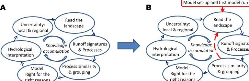
the modelling objectives. In addition, we recommend using a model that is familiar to the modeller and open for changes, allowing coherent hydrological interpretations and code ad-justments to cope with the region’s spatial heterogeneity and hydrological features. Setting up the model system includes (i) acquiring readily available data sets that cover the entire geographical domain or merge data sets to get a full cov-erage; (ii) defining calculation points and river network, by taking into account the location of gauges, major landscape features, user requests, catchment borders and routing; and (iii) making a first set of model input-data files and making the first model run for the model domain with a multi-basin resolution. The analysis of results from the first model run will indicate major obstacles, such as systematic errors in in-put data or model structural limitations. Moreover, by having the technical system in place immediately facilitates an incre-mental and agile approach to model set-up, with direct feed-back on model performance at many gauges. We then recom-mend starting to improve the performance according to the six steps of best practices for predictions in ungauged basins, using a bottom-up approach to refine input data, model struc-ture, and parameter values.

2.1 Read the landscape

Go out to your catchment, look around. . . ! (Blöschl et al., 2013, p. 385)

It is practically impossible to visit all of the basins in a large-scale domain, so instead we recommend to (i) navi-gate on hard-copy maps, digitised maps, and on the Web (e.g. Google Earth) to check landscape characteristics; (ii) review the literature for dominant processes and well-known fea-tures or hydrological challenges in the region; (iii) proceed with quality checks and cross-validations with other data sources (i.e. sources that are limited in space but contain local information); (iv) validate the basin delineation and routing using archived metadata from other available data sets; (v) check the quality of observed discharge data to assure coher-ence of time series; and, finally, (vi) check the spatiotemporal information of meteorological data sets after transformation from the grid to the subbasin scale. It is important to get an understanding of the entire domain and ensure that the data sets correspond to this understanding, hence tackling system-atic errors in the data.

2.2 Runoff signatures and processes

Analyse all runoff signatures in nearby catchments to get an understanding. . . ! (Blöschl et al. 2013, p. 385)

Detailed inspection of flow signatures for each gauging station, from large data sets (often in the range a thousand stations; see http://hypeweb.smhi.se/), is best done by using clustering techniques to discover spatial similarities (Sawicz

et al., 2011). It is then important to use many flow signatures for each site to fully capture the characteristics of the hydro-graphs. We also recommend searching for statistical relation-ships between the observed flow signatures and basin charac-teristics (both physiography and human alteration) across the model domain. This will increase our understanding of the dominant processes and fitness of the model structure (Don-nelly et al., 2015).

2.3 Process similarity and grouping

. . . find similar gauged catchments to assist in pre-dicting runoff in the ungauged basin! (Blöschl et al. 2013, p. 385)

In most process-based models, the modeller has some free-dom to define the characteristics of the smallest calculation units, which are normally linked to physiography to account for spatial distribution of for instance soil properties or land use. When producing these calculation units both technical (e.g. computational efficiency) and conceptual (e.g. restric-tions with the number of classes) concerns must be taken into account. However, lakes, wetlands, glacier, and urban areas should be respected since even small proportions can significantly alter the flow regime. When calculation units are defined, we recommend clustering the basins/gauges with similar upstream characteristics and/or system behaviour to isolate key processes for regionalisation of parameter values during calibration. We finally suggest checking the spatial distribution by plotting the catchment characteristics of sub-basins on maps and comparing them to the original or other data sources.

2.3.1 Quality checks

This is an additional step in the procedure accounting for rep-etition of steps 1–3 in an iterative way to ensure quality in the required input data and files of the model prior to pa-rameter tuning (Fig. 1); it is easy to make mistakes and in-troduce errors when handling large data sets with automatic scripts (the generalisation of scripts is not always straightfor-ward and some manual adjustment is usually required) and/or by human error (particularly when many modellers collabo-rate), which can lead to erroneous assumptions on hydrolog-ical processes during calibration. We recommend analysing flow time series as follows: (i) compare modelled to observed time series and signatures, (ii) check water-volume errors and their distribution in space, (iii) inspect the spatial distribution of model dynamics to correct spatial patterns from systematic errors, and (iv) search for errors in the model set-up (routing, meteorological input, etc.).

2.4 Model – right for the right reasons

Runoff signatures & Processes

Model: Right for the right reasons

Read the landscape Uncertainty:

local & regional

Process similarity & grouping Hydrological

interpretation

Knowledge accumulation

Runoff signatures & Processes

Model: Right for the right reasons

Read the landscape Uncertainty:

local & regional

Process similarity & grouping Hydrological

interpretation

Knowledge accumulation

A

B

Figure 1. Best practices for predictions in ungauged basins: (a) according to Fig. 13.1 by Takeuchi et al. (2013) in Blöschl et al. (2013); (b) modified version for multi-basin applications at the large scale.

catchments. . . more information than the hydro-graph. . . ! (Blöschl et al., 2013, p. 385)

Here, it is crucial that the model structure represents the modeller’s perception of how the hydrological system is or-ganised and how the various processes are interconnected. For the model set-up to be “right for the right reasons”, we recommend to: (i) constrain relevant parameters to alterna-tive data rather than just to time series of river discharge (e.g. snowmelt parameters to snow depths, evapotranspira-tion parameters to data from flux towers and satellites) or select a subset of gauges representing different flow gener-ating processes; (ii) apply expert knowledge when analysing internal variables to ensure that the model structure reflects the understanding of flow paths and their interconnections; (iii) change the model algorithms or structure if tuning of parameters is not enough to reflect the perception of the hy-drological system; (iv) include specific rating curves of lakes and reservoirs wherever available, and tune parameters for ir-rigation and dam regulation to fit the flow dynamics at down-stream gauges; and (v) if possible assimilate observed data, e.g. snow, upstream discharge, and regulation rules in reser-voirs.

2.5 Hydrological interpretation

Interpret the parameters. . . and justify their values against what was learnt during field trips and other data. . . ! (Blöschl et al., 2013, p. 385)

Although, hydrological interpretation has been present in every step of the model set-up procedure described here, this step includes the overall synthesis and analysis of results both at the large scale and for single catchments in the multi-basin approach. For spatial interpretation, we recommend plotting maps with multi-basin outputs for several variables, perfor-mance criteria, and signatures across the model domain. This allows checking the model’s coherency at various landscape features, e.g. spatial patterns of vegetation, geology, climate,

population density, and human alterations. The objective is to understand the drivers that influence flow, find rational reasons behind the hydrological heterogeneity, and identify knowledge gaps or model limitations. For temporal interpre-tation, we recommend plotting time series for some basins in each group of similar landscape units and catchment re-sponse. This is to make sure that the model reflects our per-ception and assists to better understand the dominant drivers of the flow generation processes and water dynamics in the region.

2.6 Uncertainty – local and regional

. . . by combining error propagation methods, re-gional cross-validation and hydrological interpre-tation. . . ! (Blöschl et al., 2013, p. 385)

Multi-basin models are more computationally demanding than single-basin models and it is therefore not always fea-sible to explicitly address all uncertainties from all sources. To explore the model performance in ungauged basins, we recommend dividing the set of gauging stations into those used in calibration and independent “blind-tests”, respec-tively. Cross-validation, e.g. using the jackknife procedure (Good, 2006), is practically difficult in process-based mod-elling of multi-basins. To examine uncertainties we recom-mend to (i) use several performance (diagnostic) criteria and many flow signatures, (ii) relate the spatial distribution of model performance to physiographical variables, and (iii) check model performance for independent gauging sites and new data sets.

and to make the set-up process transparent. This sets a base-line for the next round of improvements.

3 Data and methods

3.1 Study area and data description

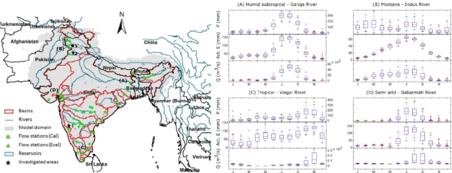
India is considered the seventh largest country by area and the second-most populous country with over 1.2 billion peo-ple. The country covers an area of about 3.3 million km2 and some of its river basins expand over several countries in the area (i.e. China, Nepal, Pakistan, and Bangladesh; see Fig. 2). The spatiotemporal variation in climate is per-haps greater than in any other area of similar size in the world. The climate is generally strongly influenced by the Hi-malayas and the Thar Desert in the northwest, both of which contribute to drive the summer and winter monsoons (Attri and Tyagi, 2010). Four seasons can be distinguished: winter (January–February), pre-monsoon (March–May), monsoon (June–September), and post-monsoon (October–December). The temperature varies between seasons ranging from mean temperatures of about 10◦C in winter to about 32◦C in the pre-monsoon season. In terms of spatial variability, the rain-fall pattern roughly reflects the different climate regimes of the country, which vary from humid in the northeast (rainfall occurs about 180 days year−1), to arid in Rajasthan (20 days year−1). Accordingly, river flow shows large spatial and seasonal variability across the subcontinent (Fig. 2b), e.g. the Ganges River has an intra-annual amplitude in monthly river discharge of 50 000 m3s−1.

For the hydrological model set-up, we use global data sets to extract the input data (see Table 1). APHRODITE (Asian Precipitation - Highly Resolved Observational Data Integra-tion Towards EvaluaIntegra-tion of the Water Resources; Yatagai et al., 2009, 2012) and AphroTEMP (Yasutomi et al., 2011) are the only long-term continental-scale data sets that contain a dense network of daily data (here only daily precipitation and mean temperature are required) for Asia including the Hi-malayas. Data of land use and soil type were aggregated into fewer classes than in the original databases. Discharge data are available from the Global Runoff Data Centre (GRDC) at 42 sites, limited to monthly values in the period 1971–1979. More discharge data are held in the Indian government agen-cies but are not accessible to the public. Consequently, in this application, flow information (Table 2) is available only for a small fraction of the subcontinent, which makes the region a great example for PUB. Monthly potential evapotranspira-tion (pot. E) data were obtained for the period 2000–2008 from the Moderate Resolution Imaging Spectroradiometer (MODIS) global data set (Mu et al., 2007, 2011). The data set covers the domain in a spatial resolution of 1 km and is derived based on the Penman–Monteith (Penman, 1948) ap-proach.

Water divides and catchment characteristics were ap-pointed for each subbasin by using the World Hydrological model Input Set-up Tool (WHIST; http://hype.sourceforge. net/WHIST/). This is a spatial information tool from SMHI (Swedish Meteorological and Hydrological Institute) to transform data and create input files for hydrological mod-els, from different types of databases. From the information of topographic databases, for example, WHIST can delin-eate the subbasins and the linking (routing) between them. This is also the tool for allocating information of soil, veg-etation, surface water, regulation and irrigation to each cal-culation unit. For the Indian subcontinent, we chose to work with some 6000 points for calculations of runoff in the river network (i.e. 6000 subbasins).

3.2 A multi-basin hydrological model for large-scale applications – the HYPE model

The HYPE model is a dynamic rainfall–runoff model which describes the hydrological processes at the catchment scale (Lindström et al., 2010). The model represents processes for snow/ice, evapotranspiration, soil moisture and flow paths, groundwater fluctuations, aquifers, human alterations (reservoirs, regulation, irrigation, abstractions), and routing through rivers and lakes. The HYPE source code is con-tinuously developed and released in new versions for open access at http://hype.sourceforge.net/, where also model de-scriptions, manuals, and file descriptions can be downloaded. HYPE is most often run at a daily time step and simu-lates the water flow paths in soil for hydrological response units (HRUs), which are defined by gridded soil and land-use classes and can be divided in up to three layers with a fluctuating groundwater table. The HRUs are further aggre-gated into subbasins based on topography. Elevation is also used to get temperature variations within a subbasin to influ-ence the snowmelt and storage as well as evapotranspiration. Glaciers have a variable surface and volume, while lakes are defined as classes with specified areas and variable volume. Lakes receive runoff from the local catchment and, if located in the subbasin outlet, also the river flow from upstream sub-basins. On glaciers and lakes, precipitation falls directly on the surface and water evaporates at the potential rate. Each lake has a defined depth below an outflow threshold. The outflow from lakes is determined by a general rating curve unless a specific one is given or if the lake is regulated. Reg-ulated lakes and man-made reservoirs are treated equally but a simple regulation rule can be used, in which the outflow is constant or follows a seasonal function (as it is often the case with hydropower) for water levels above the threshold. A rat-ing curve for the spillways can be used when the reservoir is full.

Figure 2. (Left) Map of the Indian subcontinent (model domain). Results will be shown from investigation areas with a star in the order of

their numbering. (Right) Annual cycles (1971–1979) at four river systems (a–d) of various climate (P – observed precipitation, Act.E– modelled actual evapotranspiration,Q– observed discharge).

Table 1. Data sources and characteristics of the India-HYPE v.1.0 model set-up.

Characteristic/data type Information/name Provider Total area (km2) 4.9 million – Number of subbasins 6010 (mean size 810 km2) –

Topography (routing and delineation) HydroSHEDS (15 arcsec) Lehner et al. (2008) Soil characteristics Harmonised World Soil Database (HWSD) Nachtergaele et al. (2012) Land-use characteristics Global Land Cover 2000 (GLC2000) Bartholomé et al. (2002) Reservoir and dam Global Reservoir and Dam database (GRanD) Lehner et al. (2011) Lake and wetland Global Lake and Wetland Database (GLWD) Lehner and Döll (2004) Agriculture

Irrigation

MIRCA2000

Global Map of Irrigation Areas (GMIA)

Portmann et al. (2010) Siebert et al. (2005) Siebert et al. (2010) Discharge Global Runoff Data Centre (GRDC; 42 stations) http://www.bafg.de/GRDC Precipitation APHRODITE (0.25◦×0.25◦) Yatagai et al. (2012) Temperature AphroTEMP (0.5◦×0.5◦) Yasutomi et al. (2011) PotentialE MODIS pot.E(1 km) Mu et al. (2011)

rivers, lakes, reservoirs, and/or groundwater within and/or external to the subbasin where the demands originated and are constrained by the water available at these sources. Af-ter subtraction of conveyance losses, the withdrawn waAf-ter is applied as additional infiltration to the irrigated soils. The agriculture and irrigation data sets (see Table 1) are used to define irrigated area, crop types, growing seasons, crop co-efficients, irrigation methods and efficiencies, and irrigation sources. The irrigation parameters regulating water demand and abstraction are usually manually calibrated using dis-charge stations in irrigation-dominated areas.

River discharge is routed between the subbasins along the river network and may also pass subbasins, flow laterally in the soil between subbasins or interact with a deeper ground-water aquifer in the model. For the study in this paper, the HYPE model version 4.5.0 was set up for the entire Indian

subcontinent (4.9 million km2)with a resolution of 6010 sub-basins, i.e. on average 810 km2, and is referred to as India-HYPE version 1.0.

3.3 Model calibration and regionalisation

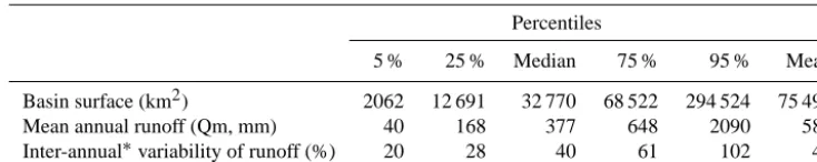
depen-Table 2. Statistics for the 42 gauging stations of river discharge used in the model evaluation.

Percentiles

5 % 25 % Median 75 % 95 % Mean Basin surface (km2) 2062 12 691 32 770 68 522 294 524 75 493 Mean annual runoff (Qm, mm) 40 168 377 648 2090 582 Inter-annual∗variability of runoff (%) 20 28 40 61 102 48

∗_{Values of inter-annual variability correspond to coefficients of variation calculated on 9-year periods.}

dent parameters) or vegetation (land-use-dependent parame-ters), while others are assumed to be general to the entire do-main (general parameters) or specific to a defined region or river (regional parameters). Parameters for each HRU are cal-ibrated for representative gauged basins and then transferred to similar HRUs, which are gridded at a higher resolution than the subbasins across the whole domain to account for spatial variability in soil and land use. Using the distributed HRU approach in the multi-basin concept is thus one part of the regionalisation method for parameter values. Some other parameters, however, are either estimated from literature ues and from previous modelling experiences (a priori val-ues) or identified in the (automatic or manual) calibration procedure. Slightly different methods for regionalisation of parameter values have been used when setting up the differ-ent HYPE model applications, depending on access to gaug-ing stations, additional data sources, and expert knowledge. The following procedure was used for India-HYPE v.1.0. 3.3.1 Stepwise, iterative calibration of parameter

groups

To tackle, to a certain extent, the equifinality problem in this processed-based model, the parameters (general, soil-and lsoil-and-use-dependent, specific or regional) are calibrated in a progressive way, i.e. stepwise calibration (Arheimer and Lindström, 2013) using different subsets of the gauging sta-tion in each step. In this way, errors induced by inappropriate parameter values in some model processes are not compen-sated for by introducing errors in other parts of the model. Hence, groups of parameters responsible for certain flow paths or processes (e.g. soil water holding capacity) are cali-brated first and then kept constant when the second group of parameters (e.g. river routing) is calibrated. However, step-ping downstream along the model code includes some recon-sideration about chosen parameter values in an iterative pro-cedure. For each step and group of parameters, a subset of representative gauging stations is used in simultaneous cal-ibration, which means that no gauging station is calibrated individually. This is to get parameters that are robust also for ungauged basins. Model performance in specific sites is thus traded against average performance across the full model do-main or regions.

For the Indian subcontinent, the following groups of HYPE parameters were calibrated stepwise: (i) general pa-rameters (e.g. precipitation and temperature correction fac-tors with elevation), which significantly affect the water bal-ance in the system, snowpack and distribution, and regional discharge; (ii) soil- and land-use-dependent parameters (e.g. field capacity and rate of potential evapotranspiration), which can influence the dynamics of the flow signal, groundwater levels, and transit time; (iii) regional parameters, which are applied as multipliers to some of the general soil and land-use parameters and may be seen as downscaling parameters as they compensate for the scaling effects and/or other types of uncertainty. The multipliers are either specific for a region or a river basin.

3.3.2 Expert knowledge for parameter constraints During this progressive stepwise calibration approach, con-straints based on expert knowledge and basin similarity are introduced. As an example, we apply a constraint imposed on the mactrsm soil dependent parameter (mactrsm is the thresh-old soil water for macropore flow and surface runoff). In the first run, during the calibration procedure the parameter is al-lowed to vary freely within the parameter range and all distri-butions for the soil types are acceptable (unconstrained sets). We then apply expert knowledge on the parameter distribu-tion and agree that a model will only be retained as feasible if it can satisfy the following constraint:

mactrsmCoarse>mactrsmMedium>mactrsmFine.

The mactrsm values for the remaining two soil types in the India-HYPE model domain, i.e. organic and shallow, are ex-pected to be close to the corresponding values for the coarse soil, although the value for shallow soil is constrained to be less than mactrsm for organic soils.

into homogeneous classes. A silhouette analysis was used to overcome the subjectivity on the determination of the num-ber of clusters. The catchment similarity approach signifi-cantly reduces the number of parameters, while it allows for regionalisation of parameters, which are assumed to be ro-bust enough also for ungauged basins.

3.3.4 Spatiotemporal calibration and evaluation India-HYPE was calibrated and evaluated in a multi-basin approach by considering the median performance in all se-lected stations. Thirty stations were sese-lected for model cal-ibration and 12 “blind” stations for spatial validation. The years 1969–1970 are used as a model warm-up period, the next 5 years for model calibration (1971–1975) and the final 4 years for temporal performance evaluation (1976–1979).

The differential-evolution Markov-chain (DE-MC; Ter Braak, 2006) optimisation algorithm is used to explore the feasible parameter space and to investigate parameter sensi-tivity. DE-MC was applied at each step of the iterative cal-ibration procedure (to optimise the general, soil- and land-use-dependent, and regional parameters) with 200 genera-tions of 100 parallel chains each being explored. The Kling– Gupta efficiency, KGE (Gupta et al., 2009), was used to de-fine the performance of the model towards the observed dis-charge. KGE allows for a multi-objective perspective by fo-cusing on separately minimising the correlation (timing) er-ror, variability erer-ror, and bias (volume) error. We also inves-tigated the relative influence of timing, variability and vol-ume error on the KGE value. To do this, we transformed the three components to result into a consistent range of possible values (the metrics are named cc, alpha and beta correspond-ing to timcorrespond-ing, variability and volume errors, respectively; see Appendix A).

3.4 Evaluation beyond standard performance metrics 3.4.1 Evaluation based on flow signatures

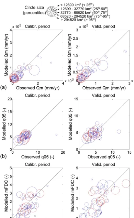
The model was further evaluated on its ability to capture spa-tial and temporal variability in discharge by comparing mod-elled flow signatures and monthly simulations with observed data. Here, three flow signatures are calculated for each gaug-ing station to illustrate the different aspects of the flow vari-ability and the hydrograph characteristics (Appendix A): the mean annual specific runoff (Qm, mm yr−1), the normalised high flow statistic (q05, –), and the slope of the flow duration curve (mFDC, –).

3.4.2 Multi-variable evaluation

To judge model credibility, observed variables other than river discharge are used, for instance from satellite prod-ucts. For India-HYPE, these included evaluations against the estimated areal extent of snow and the snow water equiva-lent from the GlobSnow system and potential

evapotranspi-ration (pot.E) from the MODIS system. The assumption is that MODIS pot. E can be used as reference to calibrate the HYPE parameters that control pot. E; this refers only to the cevp land-use-dependent parameter, which is a coef-ficient of potential evapotranspiration (mm d−1◦C−1) (Lind-ström et al., 2010). The cevp parameter was optimised for each land-use type so that the HYPE modelled annual pot. Ematches the MODIS annual pot.Eat the entire model do-main. A Monte Carlo uniform random search was used to explore the feasible cevp parameter space (constant for each land-use type; 0.15–0.30) and to investigate parameter iden-tifiability and interdependence (10 000 samples). The root mean square error (RMSE) and absolute bias (Bias) were used as objective functions in this analysis; 0 values indicate a perfect model with no errors for both criteria. Note that the analysis was conducted in the 2000–2008 period during which MODIS data were available. We therefore assume that the cevp parameter is static in time and representative also for the 1971–1979 period.

3.4.3 Linking performance to physiographical characteristics

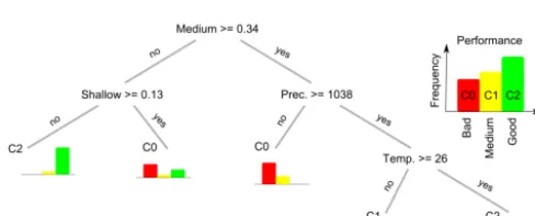
To better understand the model performance and identify po-tential for model improvements, we apply classification and regression trees (CART; Breiman et al., 1984). CART is a recursive-partitioning algorithm that classifies the space de-fined by the input variables (i.e. physiographic–climatic char-acteristics) based on the output variable (i.e. KGE model performance). The tree consists of a series of nodes, where each node is a logical expression based on a similarity met-ric in the input space (physiographic–climatic characteris-tics). In this case, we divided the KGE performance into three groups, bad (KGE < 0.4), medium (0.4 < KGE < 0.7), and good (KGE > 0.7), which were termed C0, C1, and C2, respectively. A terminal leaf exists at the end of each branch of the tree, where the probability of belonging to any of the three output groups can be inspected. Here we summarised the physiographic–climatic characteristics of the basin into five soil types (coarse, medium, fine, organic, and shallow), seven land-use types (crops, forest, open land with vegeta-tion, urban, bare/desert, glacier, and water), mean annual pre-cipitation, and mean temperature.

3.5 Catchment functioning across gradients

den-sity (–), declining limb denden-sity (–), long-term mean dis-charge (m3s−1_{), and normalised relatively low flow (–). We} then applied a k-means clustering approach within the 12-dimensional space (consisting of the 12 calculated flow sig-natures) to categorise the subbasins based on their combined similarity in flow signatures. Through the mapping of the spatial pattern we gained insight into the similarities of catch-ment functioning and could identify the dominant flow gen-erating processes for specific regions. To further highlight the hydrological insights gained during model identification, we conducted the clustering analysis on two different steps of the model calibration and explored the sensitivity of calibration on the spatial patterns of flow signatures.

4 Results and discussion

The very first model set-up to establish a technical model infrastructure of the Indian subcontinent showed very poor model performance, with an average and median KGE for all stations of−0.02 and 0.0, respectively. This performance was expected while it set the baseline for further improve-ments following the six steps of the modified PUB best prac-tices.

4.1 Read the landscape

Background knowledge was firstly acquired via visual and/or numerical analysis of available maps that describe the spa-tial patterns of land use, soil, and climate, as well as via the study of the scientific literature on regional hydrologi-cal investigations, which enabled identification of dominant physical processes and flow paths. Such soft information was useful for turning processes on/off and selecting relevant al-gorithms, e.g. for management and snow melting. Commu-nication with local scientists (i.e. governmental hydrological institutes), managers (i.e. regional water authorities) and end-users (i.e. agricultural sector) enabled knowledge exchange and justified the model approach. Three extensive field trips provided important soft information about system behaviour in the semi-arid northwest and humid subtropical northeast-ern parts of the country (i.e. identification of irrigation water sources for agricultural needs and estimation of water losses due to faults in the irrigation systems).

Analyses of the topographic data were of major impor-tance since they affected the subbasin delineation and rout-ing. Although HydroSHEDS (Hydrological data and maps based on SHuttle Elevation Derivatives at multiple Scales) is based on high-resolution elevation layers, which are hydro-logically conditioned and corrected, there are still many er-rors. Merging HydroSHEDS with GRDC (hence forcing the delineation at subbasins where GRDC stations are available) involved some mismatches in terms of the size of upstream areas between the subbasin delineations and the GRDC meta-data. As an example, the location of the Dandeli station in

the Kali Nadi River basin (asterisk 1 in Fig. 2) was adjusted to match the underlying topography and drainage accumula-tion data based on published and computed upstream areas, respectively (see Fig. 3a). The consequent change in the rout-ing resulted in a considerable improvement in the model per-formance (KGE improved from−0.51 to 0.30; see Fig. 3b). Many similar corrections had to be made.

To make corrections also for ungauged basins and major rivers, the delineated basins were additionally evaluated us-ing a shapefile of basin areas reported by Gosain et al. (2011). Some minor corrections had to be done in the routing to achieve similarly delineated basins, particularly in the north-western region, where mean elevation at the subbasin scale does not show much variability.

4.2 Runoff signatures and processes

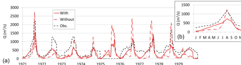
As recommended, several flow signatures were extracted from the gauging stations across India to be compared to physiographical patterns. Flow signatures were also used for model evaluation to find potential for improvements. The analysis was done at different stages in the model set-up and, finally, there was a relatively good agreement of the observed and modelled flow signatures (Fig. 4). In general, poor agree-ment was found in mountains and in semi-arid regions, which are characterised by local, convective rainfall events during the monsoon season. No clear pattern is found between sig-nature agreement and basin scale for calibrated river gauges. We also explored how flow signatures can be affected by human impacts by analysing modelled responses consider-ing and omittconsider-ing the human influence. Figure 5 highlights the significant effect reservoirs have to dampen hydrographs and control discharge variability, hence various flow signatures. The model can represent fairly well the reservoir routing and KGE improved from 0.37 to 0.48 after introducing a regula-tion scheme. The model improved on capturing the seasonal-ity of regulation; however, at this modelling state it was not able to represent the monthly peaks. Note that model results are subject to the general rating curve generalised to all reser-voirs; there were no downstream data available to calibrate the parameters specifically for a given reservoir/dam. 4.3 Process similarity and grouping

Figure 3. Example of the impact of basin delineation and routing on model behaviour: (a) correction in the location (red x and green circle

is prior and after the correction, respectively) of the Dandeli discharge station (Kali Nadi River basin) and (b) the corresponding modelled discharge before and after the correction. In (a) the subbasins and flow accumulation are also depicted.

Figure 4. Signature analysis in the spatiotemporal model

evalua-tion: (a) the mean annual specific runoff, (b) the normalised high flow statistic, and (c) the slope of the flow duration curve. Blue and red circles are used for the calibration and evaluation stations, re-spectively.

characteristics had more influence on the clustering as op-posed to the climatic properties; the clustering was repeated without climatic information but the spatial pattern of the clusters remained. In the last stage of the stepwise calibration procedure, the regional model parameters were estimated for each cluster region. Using the clustering for regional cali-bration (Sect. 5.4), however, could not significantly improve the overall model performance but, nevertheless, the model consistency at all stations was improved. Overall, we found a high number of potential catchment similarity concepts to drive parameter identification in the ungauged basins. 4.3.1 Quality checks

Steps 1–3 of our best practices were performed in an itera-tive procedure including checking against independent data sources that resulted in the reconsideration of assumptions and corrections of input data. For instance, the proportion of each land-use type driven by GLC2000 was calculated and compared to soft information from official governmental re-ports. According to GLC2000 11 % of the country is forest, which contradicts the estimated 22 % based on reports from the Ministry of Water Resources (India-WRIS, 2012; River Basin Atlas of India, RRSC-West, NRSC, ISRO, Jodpur, In-dia). To address this, forest information from the Global Ir-rigated Area Mapping (GIAM; Thenkabail et al., 2009) was merged with GLC2000. Although the proportion of forest ar-eas was corrected, this merging consequently changed the proportion of open land with vegetation and crops from 14 and 68 % to 12 and 59 %, respectively.

In-Figure 5. Impact of model parameterisation of reservoir regulation on discharge for (a) monthly streamflow, and (b) annual hydrograph,

showing naturalised (without) and regulated (with) conditions at the basin outlet (located at asterisk 2 in Fig. 2).

Figure 6. Subbasin clusters using a k-means clustering approach based on physiographical characteristics.

dian Meteorological Department showed an underestimation of the APHRODITE precipitation in the mountainous re-gions: the APHRODITE precipitation network is sparse over the Himalayas (Yatagai et al., 2012). To overcome this un-derestimation, a correction factor was applied to precipita-tion (in HYPE, this was a multiplier of 4 % per 100 m) at regions with elevation greater than 400 m. By allowing such modification in the data, we expected that the calibration of model parameters could further compensate for precipitation uncertainty.

4.4 Model – right for the right reasons

When setting up India-HYPE we considered realism in the process calculations by using parameter constraints. We did not have to adjust the model structure and we did not assim-ilate data or rating curves as we did not have access to such observations.

Crops Forest Open land veg. Urban Desert Glacier Lake 0.15

0.20 0.25 0.30

cevp

RMSE Bias

Figure 7. Coefficient of potential evapotranspiration (cevp)

param-eter as identified (the range is derived from the 100 paramparam-eter sets that perform best, and the optimum set) for different objective functions (RMSE and Bias) and land-use type. Lines with markers present the optimum parameter values for different objective func-tions.

4.4.1 Additional data sources

The calibration of the pot. E model routine against the MODIS pot.Edata resulted in a well-identified cevp value for most land-use types. Analysis of the Monte Carlo re-sults presents an initial screening of parameter sensitivities (Fig. 7). Results show that the different objective functions extract different information from the pot.Espatial pattern. As expected, cevp values for crops, forest, and open land with vegetation types are the most sensitive to both objec-tive functions, since these land-use types dominate the region (60, 23, and 11 % of India, respectively) and hence signifi-cantly affect pot.E. Overall, India-HYPE was lower in pot. Eat the arid regions and over the Himalayas (on average by 15 %), whereas it was higher in pot.Ealong the western and eastern coastlines (on average by 12 %). Although the two estimates do not fully match, the use of additional informa-tion to constrain parameters (hence constraining the model’s results for specific processes) is promising. However, the un-certainty of MODIS results was not examined and more data sources should be included.

4.4.2 Expert knowledge

mod-0" 0.5" 1"

Coarse" Medium" Fine" Organic" Shallow"

m

ac

tr

sm

"

Constrained" Unconstrained"

Figure 8. Constraints (grey dashed lines) and optimum (solid lines)

values of the mactrsm soil-dependent model parameter based on process understanding.

els resulted in a comparable calibration performance: me-dian KGE was 0.48 and 0.49 for the constrained and uncon-strained models, respectively. The optimum set for the un-constrained model gave an unrealistic distribution of the pa-rameter values for the coarse and medium soil types (Fig. 8). However, the optimum values are within the parameter range defined in the constrained calibration approach. The slight increase is due to the free calibration parameters whose val-ues and/or distributions are allowed to compensate for er-rors/uncertainties at other processes. In such cases it is im-portant to select the model which performs well and respects the theoretical understanding of the system. This illustrates the value of the recommendations to constrain parameters based on expert knowledge – the right model for the right reason.

4.4.3 Stepwise calibration procedure

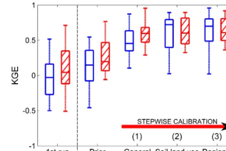
The predictability of the model with prior parameter values was very poor (Fig. 9), highlighting the limitations when pa-rameters are regionalised from a donor system of strongly different hydroclimatic characteristics (e.g. Sweden). A sig-nificant improvement in the performance is achieved in both the calibration and the evaluation period after the calibra-tion of the general parameters due to a better representacalibra-tion of the water volume in the rivers (beta in KGE improved from 0.51 to 0.78). Calibration of the soil and land-use pa-rameters further improved the overall performance; however, KGE slightly decreased at the basins in which the model per-formed poorly during the previous calibration step. Using the clusters based on catchment similarities for regional calibra-tion did not significantly improve the overall model perfor-mance; however, the model consistency at all stations was improved in both calibration and evaluation periods. 4.5 Hydrological interpretation

The temporal interpretation was done by analysing interact-ing dynamics of internal model variables, i.e. precipitation (P, mm), snow depth (SD, mm), temperature (T,◦C), evap-otranspiration (E, mm), soil moisture deficit (SMDF, mm), and discharge (Q, m3s−1). These are checked visually in a set of validation basins, to avoid unrealistic model behaviour

Figure 9. Improvements in model performance (average KGE for

30 stations) during the stepwise calibration approach (steps 1–3 cor-respond to general, soil-land use, and regional calibration as de-scribed in Sect. 3.3). “1st run” corresponds to model performance of the very first model set-up to establish a technical model infras-tructure. “Prior” corresponds to model performance before param-eter calibration and after overcoming routing errors. The evaluation is conducted at the calibration (blue) and the validation (red shaded) period.

due to parameter setting. Results from this point onwards correspond to the calibrated India-HYPE model (after step 3 in Fig. 9). Results in the Chenab River at the Akhnoor sta-tion (branch river of the Indus system; asterisk 3 in Fig. 2) show that the snowmelt characterises the monthly hydro-graph (Fig. 10). Snow accumulation/melting processes occur at the headwaters of the basin which experience T below 0◦_C

during the winter and pre-monsoon period and above 0◦_C

during the rest of the months (“Up” black-dashedT series in Fig. 10).P also varies in space while it exhibits strong seasonal variability according to the location (“Up” black-line and “Down” blue envelope in theP series). Spatiotem-poral analysis ofP allows for a better understanding of the snow depth temporal distribution; in the model, snow depth increases when precipitation occurs and temperature is below 0◦C. Given the model’s evapotranspiration module, potential Evaries depending on mean temperature. However the dis-tribution of actualEis dependent on the water availability in the soil, which further justifies the strong (negative) correla-tion between actualEand SMDF.

in-Figure 10. Analysis of model variables at the Akhnoor station (Chenab River; asterisk 3 in Fig. 2):P, SD,T,E, SMDF andQ.Ecorresponds to potential (Pot.) and actual (Act.) evapotranspiration, andQcorresponds to modelled (Mod.) and observed (Obs.) discharge). Note thatP

andT series are plotted at the outlet of the basin (Down) and the most upstream subbasin (Up).

Figure 11. Classification trees relating regions of different KGE

performance with physical and climatic characteristics. The bars represent the probability of a performance resulting in any of the three performance classes (C0, C1 or C2).

sightful and show that poor performance (KGE < 0.4) is gen-erally achieved at basins with shallow soil type greater than 13 %. The probability of obtaining poor performance is also highest for basins with medium soil type greater than 34 % and precipitation less than 1038 mm. Consequently, empha-sis should be given to parameters for medium and shallow soils in a future effort to improve the model performance. 4.6 Uncertainty – local and regional

The India-HYPE model was calibrated and validated in space and time, and the overall model performance (at the end of the stepwise approach) in terms of KGE (Gupta et al., 2009)

and its decomposed terms is presented in Table 3. India-HYPE achieved an acceptable performance and is therefore considered adequate to describe the dominant hydrological processes in the subcontinent. However, the performance de-creased (from KGE=0.64 to KGE=0.44) when the model was evaluated for gauges, which are independent both in space and time. This shows that the model still needs im-provements to be equally reliable for predictions in ungauged basins at independent time periods. The decomposed KGE terms show that the model, during the validation period and for the validation stations, cannot fully capture the variabil-ity of the observed data (described by the alpha term). Alpha decreases during the validation period at the validation sta-tions from 0.78 to 0.58, which consequently affects the KGE values. However, other flow characteristics, i.e. timing and volume, are well represented also during the validation pe-riod.

Table 3. Median model performance for calibration and validation stations and periods.

Space Time KGE cc (timing) alpha (variability) beta (volume) Cal. (30 stations) Cal. (1971–1975) 0.64 0.93 0.78 0.75

Val. (1976–1979) 0.62 0.92 0.81 0.80 Val. (12 stations) Cal. (1971–1975) 0.64 0.91 0.78 0.79 Val. (1976–1979) 0.44 0.84 0.58 0.75

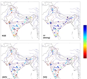
KGE’s decomposed terms (cc, alpha and beta) can reveal the causes for the model errors. For example, the poor perfor-mance at the Indus river system (northern India) is due to the poor representation of the observed variability of discharge, which is probably related to parameterisation in the model’s snow accumulation/melting component. In addition, a mass volume error seems to be the main cause of the poor KGE performance in the southwestern rivers. This seems to be due to the underestimation of precipitation and/or overestimation of actual evapotranspiration: a comparison of APHRODITE data against precipitation data from the Indian Meteorolog-ical Department showed underestimation of precipitation in this region. Conclusions are similar for the stations used in the calibration and validation analysis, hence justifying the model’s spatial consistency in the region.

4.7 Spatial flow pattern across the subcontinent and dominant processes

Although the India-HYPE model has limitations, we identi-fied potential for further improvements during the set-up pro-cedure. The present version has demonstrated the usefulness of multi-basin modelling for comparative hydrology and how to gain insights in spatial patterns of flow generating pro-cesses at the large scale. The final clustering analysis of the 12 flow signatures from India-HYPE version 1 resulted in six different classes of varying size (Fig. 13) with different dis-tributions in the signatures (Fig. 14). Similarity in catchment behaviour for each class was interpreted and dominant flow generating processes could be distinguished as follows.

Catchments in cluster 3 are located in the Himalayan re-gion and in the western Indian coast (Western Ghats) and are characterised by high ranges of annual specific runoff (Qm) due to high precipitation occurring in these regions, and vari-able flow regime (high mFDC). Variability is dependent on snow/ice processes which are important in controlling the flow regime, at least in the Himalayan region (cf. annual cy-cle in the Indus River in Fig. 2). Flow is also characterised by high rising and declining limb densities (RLD and DLD). The climate in catchments of cluster 3 is humid subtropical and tropical with high evapotranspiration. Catchments in the northwestern part of India (cluster 4; arid regions including the Thar Desert) are characterised by high intra-annual vari-ability (DPar) and low values of flow (q95). Ephemeral rivers exist in this region due to high evaporation rates (e.g. the Luni

River), and generate runoff mainly during the monsoon pe-riod. The high variability in the flow regime is also shown by the high values of CV (coefficient of variation), flash and RLD signatures. Similar flow characteristics are observed for the catchments located in the semi-arid regions (cluster 1), yet not at the same range of signature values as for cluster 4. The catchments in cluster 1 are also fast, responsive and their flow shows strong dynamics, in terms of RLD and DLD. Catchments in cluster 2 are located in the tropical climate and their runoff response is mainly driven by rainfall. Al-though these catchments receive less precipitation compared to other regions, their normalised high flow statistic (q05) is the highest of any cluster group. Moreover, catchments in cluster 5 are located at the downstream areas of the Indus River, distinguished for their high values of low flows. Fi-nally, catchments in cluster 6 are characterised for their high mean annual discharge values and are located at the down-stream areas of the large river systems (Indus, Ganges and Brahmaputra). Note also that only few catchments belong to these cluster groups: 112 and 57 catchments in clusters 5 and 6, respectively.

Figure 12. Spatial variability of KGE (and its decomposed terms) model performance for the calibration (circle) and validation (triangle)

stations.

Figure 13. Subbasin clusters based on flow signatures at different stages of the model set-up: (a) prior, and (b) regional.

4.8 Performance in India-HYPE v1.0 and future model refinements

Many other catchment-scale and multi-basin hydrological models have been applied in (parts of) the Indian subcon-tinent. However, it is generally common that only results

guide-Figure 14. Distribution of signature values for each cluster (at the regional step). The flow signatures are described in Appendix A.

lines on how to start working on the next version, loop-ing back to step 1. Overall, India-HYPE performed well for most river systems, with the performance being comparable to other studies in which a model was applied at the large scale. Application of the VIC (Variable Infiltration Capacity) hydrological model resulted in a similar performance for the large systems of the Ganges, Krishna, and Narmada (Raje et al., 2013) with the Nash–Sutcliffe efficiency, NSE (Nash and Sutcliffe, 1970), varying between 0.44 and 0.94 (at the same stations India-HYPE achieved an NSE between 0.45 and 0.94). In contrast to previous studies, our contribution lies in the fact that anthropogenic influences (i.e. reservoirs and irrigation) are simulated, as those have been shown to be very important in controlling the amplitude, phase, and shape of the hydrograph. Other models, e.g. SWAT, have also been applied in India to assess the impacts of climate change; how-ever, the parameters have been estimated empirically from the literature, whilst the performance was not reported (Go-sain et al., 2006, 2011).

Catchment-scale hydrological models from India have generally been achieving a high performance (Arora, 2010; Patil et al., 2008), mainly due to the local gauged data used: usually the data are governmental and confidential with high spatiotemporal resolution and less uncertainty/error. In addition, model parameters in single catchments are nor-mally transferred along a smoother hydroclimatic gradient and are calibrated for individual gauging stations. Never-theless, catchment-scale studies set a benchmark of perfor-mance and provide deeper knowledge of process description,

5 Conclusions

By investigating the modified recommendations for predic-tions in ungauged basins across the Indian subcontinent, we found the following.

– Each step in the best-practice procedure was relevant and we could find methods that also work at the large scale using the knowledge derived for catchments dur-ing the PUB decade. We argue for adaptdur-ing an incmental and agile approach to model set-up, which re-quires frequent testing to get feedback on introduced changes. The large-scale modelling is more prone to technical problems and data inconsistencies that be-come apparent when running the model and therefore should be resolved early in the model set-up process. – Multi-basin modelling of ungauged rivers at the large

scale reveals insights into spatial patterns and domi-nating flow processes. Indian catchments can be cate-gorised into six clusters based on their flow similarity. River flow varies spatially in terms of flow means, vari-ability, extremes, and seasonality. Catchments in the Hi-malayan region and the Western Ghats seem to respond similarly and are characterised by high mean annual specific runoff values and variable flow regime. The re-sponse of the catchments in the tropical zone is char-acterised by high peaks, while catchments in the dry regions show very strong flow variability and respond quickly to rainfall.

Appendix A: Definition of performance metrics and flow signatures

The Kling–Gupta efficiency (KGE) is defined as KGE=1−

q

(r−1)2_+(α−1)2_+(β−1)2_,

whereris the linear cross-correlation coefficient between ob-served and modelled records,αis a measure of variability in the data values (equal to the standard deviation of modelled over the standard deviation of observed), and β is equal to the mean of modelled over the mean of observed records. For a perfect model with no data errors, the value of KGE is 1; hencer,α, andβ are also 1. In addition, we transform the three KGE components to results in a consistent range of possible values. Consequently, we consider

cc=1−p(r−1)2, alpha=1−p(α−1)2, beta=1−p(β−1)2,

where the range of values for each term varies between−∞ and 1 with 1 being the optimum.

In this paper we quantify the signatures by single values. Given the time series of observed (or modelled) specific daily runoffQd(t )(mm d−1), the calculated signatures are given in Table A1.

Table A1. Flow signatures used for model evaluation and catchment

functioning.

Signature Abbreviation Reference

Acknowledgements. We are very grateful for the funding of this

research by the Swedish International Development Cooperation Agency (Sida) through the India-HYPE project (AKT-2012-022) and the Swedish Research Council (VR) through the WaterRain-Him project (348-2014-33). The investigation was performed at the SMHI Hydrological Research unit, where much work is done jointly. We would especially like to acknowledge contributions from David Gustafsson, Göran Lindström, Jafet Andersson, Kean Foster, Kristina Isberg, and Jörgen Rosberg for assistance with background material for this study. The authors would finally like to express their sincere gratitude to two anonymous reviewers for their constructive comments. Their detailed suggestions have resulted in an improved manuscript. The open-source HYPE model code can be retrieved with its manuals at http://hype.sourceforge.net/. Time series and maps from the India-HYPE model (including climate change impact studies) are available for inspection at http://hypeweb.smhi.se. The work contributes to the decadal research initiative Panta Rhei by the International Association of Hydrological Sciences (IAHS) under Target 2, Estimation and Prediction, and its two working groups on large samples and multiple ungauged basins, respectively.

Edited by: R. Woods

References

Alcamo, J., Döll, P., Henrichs, T., Kaspar, F., Lehner, B., Rösch, T., and Siebert, S.: Development and testing of the WaterGAP 2 global model of water use and availability, Hydrolog. Sci. J., 48, 317–337, doi:10.1623/hysj.48.3.317.45290, 2003.

Allen, R. G., Pereira, L. S., Raes, D., and Smith, M.: Crop evapo-transpiration, Guidelines for computing crop water requirements, in FAO Irrigation and drainage paper, Rome, 56, 1998.

Andreassian, V., Hall, A., Chahinian, N., and Schaake, J.: Large Sample Basin Experiment for Hydrological Model Parameteri-zation: Results of the Model Parameter Experiment – MOPEX, IAHS Publication, Wallingford, 307, 2006.

Arheimer, B. and Brandt, M.: Modelling nitrogen transport and re-tention in the catchments of southern Sweden, Ambio, 27, 471– 480, 1998.

Arheimer, B. and Lindström, G.: Implementing the EU Water Framework Directive in Sweden, in: Runoff Predictions in Un-gauged Basins – Synthesis across processes, places and scales, edited by: Blöschl, G., Sivapalan, M., Wagener, T., and Viglione, A., 353–359, Cambridge University Press, Cambridge, UK, 2013.

Arheimer, B., Dahné, J., Lindström, G., Marklund, L., and Strömqvist, J.: Multi-variable evaluation of an integrated model system covering Sweden (S-HYPE), IAHS Publ., 345, 145–150, 2011.

Arora, M.: Estimation of melt contribution to total streamflow in river Bhagirathi and river DhauliGanga at Loharinag Pala and Tapovan Vishnugad project sites, J. Water Resour. Prot., 02, 636– 643, doi:10.4236/jwarp.2010.27073, 2010.

Attri, S. D. and Tyagi, A.: Climate profile of India, in Government of India Ministry of Earth Sciences, New Delhi, p. 129, 2010. Bartholomé, E., Belward, A. S., Achard, F., Bartalev, S., Carmona

Moreno, C., Eva, H., Fritz, S., Grégoire, J.-M., Mayaux, P., and

Stibig, H.-J.: GLC 2000 Global Land Cover mapping for the year 2000, European Commission, DG Joint Research Centre, EUR 20524 EN, Ispra, 2002.

Blöschl, G., Sivapalan, M., Wagener, T., Viglione, A., and Savenije, H.: Runoff prediction in ungauged basins. Synthesis across pro-cesses, places and scales, Cambridge University Press, Cam-bridge, UK, 2013.

Breiman, L., Friedman, J. H., Olshen, R. A., and Stone, C. J.: Classi-fication and Regression Trees, CRC Press, Wadsworth, Belmont, CA, 1984.

Bulygina, N., McIntyre, N., and Wheater, H.: Conditioning rainfall-runoff model parameters for ungauged catchments and land man-agement impacts analysis, Hydrol. Earth Syst. Sci., 13, 893-904, doi:10.5194/hess-13-893-2009, 2009.

Bulygina, N., Ballard, C., McIntyre, N., O’Donnell, G., and Wheater, H.: Integrating different types of information into hy-drological model parameter estimation: Application to ungauged catchments and land use scenario analysis, Water Resour. Res., 48, W06519, doi:10.1029/2011WR011207, 2012.

Coron, L., Andréassian, V., Perrin, C., Lerat, J., Vaze, J., Bourqui, M., and Hendrickx, F.: Crash testing hydrological models in contrasted climate conditions: an experiment on 216 Australian catchments, Water Resour. Res., 48, W05552, doi:10.1029/2011WR011721, 2012.

Donnelly, C., Rosberg, J., and Isberg, K.: A validation of river rout-ing networks for catchment modellrout-ing from small to large scales, Hydrol. Res., 44, 917–925, doi:10.2166/nh.2012.341, 2013. Donnelly, C., Andersson, J. C. M., and Arheimer, B.: Using flow

signatures and catchment similarities to evaluate the E-HYPE multi-basin model across Europe, Hydrolog. Sci. J., in press, doi:10.1080/02626667.2015.1027710, 2015.

Euser, T., Winsemius, H. C., Hrachowitz, M., Fenicia, F., Uhlen-brook, S., and Savenije, H. H. G.: A framework to assess the realism of model structures using hydrological signatures, Hy-drol. Earth Syst. Sci., 17, 1893–1912, doi:10.5194/hess-17-1893-2013, 2013.

Falkenmark, M. and Chapman, T.: Comparative hydrology: An eco-logical approach to land and water resources, UNESCO, Paris, France, 1989.

Fenicia, F., Savenije, H. H. G., Matgen, P., and Pfister, L.: Understanding catchment behavior through stepwise model concept improvement, Water Resour. Res., 44, 1–13, doi:10.1029/2006WR005563, 2008.

Finger, D., Pellicciotti, F., Konz, M., Rimkus, S., and Burlando, P.: The value of glacier mass balance, satellite snow cover images, and hourly discharge for improving the performance of a physi-cally based distributed hydrological model, Water Resour. Res., 47, W07519, doi:10.1029/2010WR009824, 2011.

Gao, H., Hrachowitz, M., Fenicia, F., Gharari, S., and Savenije, H. H. G.: Testing the realism of a topography-driven model (FLEX-Topo) in the nested catchments of the Upper Heihe, China, Hy-drol. Earth Syst. Sci., 18, 1895–1915, doi:10.5194/hess-18-1895-2014, 2014.

Good, P. I.: Resampling methods: A practical guide to data analysis, 3rd Edn., Birkhäuser, Boston, 2006.