Hydrol. Earth Syst. Sci., 17, 2147–2159, 2013 www.hydrol-earth-syst-sci.net/17/2147/2013/ doi:10.5194/hess-17-2147-2013
© Author(s) 2013. CC Attribution 3.0 License.
EGU Journal Logos (RGB)
Advances in
Geosciences
Open Access
Natural Hazards
and Earth System
Sciences
Open AccessAnnales
Geophysicae
Open AccessNonlinear Processes
in Geophysics
Open AccessAtmospheric
Chemistry
and Physics
Open AccessAtmospheric
Chemistry
and Physics
Open Access DiscussionsAtmospheric
Measurement
Techniques
Open AccessAtmospheric
Measurement
Techniques
Open Access DiscussionsBiogeosciences
Open Access Open Access
Biogeosciences
Discussions
Climate
of the Past
Open Access Open Access
Climate
of the Past
Discussions
Earth System
Dynamics
Open Access Open Access
Earth System
Dynamics
DiscussionsGeoscientific
Instrumentation
Methods and
Data Systems
Open Access
Geoscientific
Instrumentation
Methods and
Data Systems
Open Access DiscussionsGeoscientific
Model Development
Open Access Open Access
Geoscientific
Model Development
DiscussionsHydrology and
Earth System
Sciences
Open AccessHydrology and
Earth System
Sciences
Open Access DiscussionsOcean Science
Open Access Open Access
Ocean Science
DiscussionsSolid Earth
Open Access Open Access
Solid Earth
Discussions
The Cryosphere
Open Access Open Access
The Cryosphere
DiscussionsNatural Hazards
and Earth System
Sciences
Open Access
Discussions
Errors in climate model daily precipitation and temperature output:
time invariance and implications for bias correction
E. P. Maurer1, T. Das2, and D. R. Cayan3
1Civil Engineering Dept., Santa Clara University, Santa Clara, CA, USA 2CH2MHill, 402 W. Broadway, San Diego, CA, USA
3Division of Climate, Atmospheric Sciences, and Physical Oceanography, Scripps Institution of Oceanography and Water Resources Division, US Geological Survey, La Jolla, CA, USA
Correspondence to: E. P. Maurer ([email protected])
Received: 21 December 2012 – Published in Hydrol. Earth Syst. Sci. Discuss.: 1 February 2013 Revised: 7 May 2013 – Accepted: 12 May 2013 – Published: 7 June 2013
Abstract. When correcting for biases in general circulation model (GCM) output, for example when statistically down-scaling for regional and local impacts studies, a common as-sumption is that the GCM biases can be characterized by comparing model simulations and observations for a histor-ical period. We demonstrate some complications in this as-sumption, with GCM biases varying between mean and ex-treme values and for different sets of historical years. Daily precipitation and maximum and minimum temperature from late 20th century simulations by four GCMs over the United States were compared to gridded observations. Using random years from the historical record we select a “base” set and a 10 yr independent “projected” set. We compare differences in biases between these sets at median and extreme percentiles. On average a base set with as few as 4 randomly-selected years is often adequate to characterize the biases in daily GCM precipitation and temperature, at both median and ex-treme values; 12 yr provided higher confidence that bias cor-rection would be successful. This suggests that some of the GCM bias is time invariant. When characterizing bias with a set of consecutive years, the set must be long enough to ac-commodate regional low frequency variability, since the bias also exhibits this variability. Newer climate models included in the Intergovernmental Panel on Climate Change fifth as-sessment will allow extending this study for a longer obser-vational period and to finer scales.
1 Introduction
The prospect of continued and intensifying climate change has motivated the assessment of impacts at the local to re-gional scale, which entails the prerequisite use of down-scaling methods to translate large-scale general circulation model (GCM) output to a regionally relevant scale (Carter et al., 2007; Christensen et al., 2007). This downscaling is typ-ically categorized into two types: dynamical, using a higher resolution climate model that better represents the finer-scale processes and terrain in the region of interest; and statisti-cal, where relationships are developed between large-scale climate statistics and those at a fine scale (Fowler et al., 2007). While dynamical downscaling has the advantage of producing complete, physically consistent fields, its com-putational demands preclude its common use when using multiple GCMs in a climate change impact assessment. We thus focus our attention on statistical downscaling, and more specifically on the bias correction inherently included in it.
removing the bias during an observed period and applying the same bias correction into the future should produce a projection into the future with lower bias as well. Ultimately this would place all GCM projections on a more or less equal footing.
Some past studies support the assumption of time-invariant GCM biases in bias correction schemes. For ex-ample, Macadam et al. (2010), who demonstrate that using GCM abilities to reproduce near-surface temperature anoma-lies (where biases in mean state are removed) was found to produce inconsistent rankings (from best to worst) of GCMs for different 20 yr periods in the 20th century. However, Macadam et al. (2010) found when actual temperatures were used to assess model performance, a more stable GCM rank-ing was produced. While studyrank-ing regional climate model biases, Christensen et al. (2008) found systematic biases in precipitation and temperature related to observed mean val-ues, although the biases between different subsets of years increased when they differed in temperature by 4–6◦C.
Biases in GCM output have been attributed to various cli-mate model deficiencies such as the coarse representation of terrain (Masson and Knutti, 2011), cloud and convective pre-cipitation parameterization (Sun et al., 2006), surface albedo feedback (Randall et al., 2007), and representation of land-atmosphere interactions (Haerter et al., 2011) for example. Some of these deficiencies, as persistent model characteris-tics, would be expected to result in biases in the GCM output that are similar during different historical periods and into the future. For example, errors in GCM simulations of tem-perature occur in regions of sharp elevation changes that are not captured by the coarse GCM spatial scale (Randall et al., 2007); these errors would be expected to be evident to some degree in model simulations for any time period. However, as Haerter et al. (2011) state “. . . bias correction cannot correct for incorrect representations of dynamical and/or physical processes . . . ”, which points toward the issue of some GCM deficiencies producing different biases in land surface vari-ables as the climate warms, generically referred to as time-and state-dependent biases (Buser et al., 2009; Ehret et al., 2012). For example, Hall et al. (2008) show that biases in the representation of spring snow albedo feedback in a GCM can modify the summer temperature change sensitivity. This implies that as global temperatures climb in future decades, some biases could be amplified by this feedback process. While we do not assess the sources of GCM biases explic-itly, we aim to examine where different GCMs exhibit simi-lar precipitation and temperature biases between two sets of independent years, which may carry implications as to which sources of error are important in different regions.
Many of the prior assessments of GCM bias have been based on GCM simulations of monthly, seasonal, or an-nual mean quantities. Recognizing the important role of ex-treme events in the projected impacts of climate change (Christensen et al., 2007), statistical downscaling of daily GCM output can been used to provide information on the
projected changes in regional extremes (e.g., B¨urger et al., 2012; Fowler et al., 2007; Tryhorn and DeGaetano, 2011). While accounting for biases at longer timescales, such as monthly, can reduce the bias in daily GCM output, the daily variability of GCM output may have biases (such as exces-sive drizzle; e.g., Piani et al., 2010) that cannot be addressed by a correction at longer timescales. By addressing biases at the daily scale, we can assess the ability to correct for biases at a timescale appropriate for many extreme events (Frich et al., 2002).
Biases in daily GCM output can be removed in many ways. At its simplest, the perturbation, or “delta” method shifts the observed mean by the GCM simulated mean change, effectively accounting for GCM mean bias only (Hewitson, 2003), which is useful but has its limitations (Ballester et al., 2010). Separate perturbations can be applied to different magnitude events (e.g., Vicuna et al., 2010) to capture some of the potentially asymmetric biases in differ-ent portions of the observed probability distribution function. In its limit, perturbations can be applied along a continu-ous distribution, resulting in a quantile mapping technique (Maraun et al., 2010; Panofsky and Brier, 1968). This type of approach has been applied in a variety of formulations for bias correcting monthly and daily climate model outputs (e.g., Abatzoglou and Brown, 2012; Bo´e et al., 2007; Ines and Hansen, 2006; Li et al., 2010; Piani et al., 2010; Themeßl et al., 2012; Thrasher et al., 2012), and has been shown to compare favorably to other statistical bias correction meth-ods (Lafon et al., 2012). Regardless of the approach, all of these methods of bias removal assume that biases relative to historic observations will be the same during the projections. For this study, we examine the biases in daily GCM out-put over the conterminous United States. We address the fol-lowing questions: (1) are the daily biases the same between median and extreme values? (2) Are biases the same over different randomly selected sets of years (i.e., time invari-ant)? We address these using daily output from four GCMs for precipitation, and maximum and minimum daily temper-ature. We consider biases at both median and extreme values because, as attention focuses on extreme events such as heat waves, peak energy demand, and floods, the assumptions in bias correction of daily data at these extremes becomes at least as important as at mean conditions.
2 Methods and data
Table 1. GCM names and runs used in this study.
Modeling Group GCM Name Model Runs Primary Reference
Centre National de Recherches Meteorologiques, France CNRM CNRM CM3: 20c3m run 1 Salas-M´elia et al. (2005) Geophysical Fluid Dynamics Laboratory, USA GFDL GFDL 2.1: 20c3m run 1 Delworth et al. (2006) National Center for Atmospheric Research, USA PCM NCAR PCM1: 20c3m run 2 Washington et al. (2000) National Center for Atmospheric Research, USA CCSM NCAR CCSM3: 20c3m run 5 Kiehl et al. (1998)
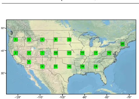
Fig. 1. Location of the 20 grid cells used in this analysis.
in California and the Western United States (Pierce et al., 2013). All GCMs were regridded onto a common 2-degree grid to allow direct comparisons of model output. While this coarse resolution inevitably results in a reduction of daily ex-tremes that would be experienced at smaller scales due to effects of spatial averaging (Yevjevich, 1972), GCM-scale daily extremes are widely used to characterize projected fu-ture changes in important measures of impacts (Tebaldi et al., 2006).
As an observational baseline the 1/8 degree Maurer et al. (2002) data set for the 1950–1999 period was used, which was aggregated to the same 2-degree spatial resolution as the GCMs. This data set consists of gridded daily cooperative observer station observations, with precipitation rescaled (us-ing a multiplicative factor) to match the 1961–1990 monthly means of the widely-used PRISM data set (Daly et al., 1994), which incorporates additional data sources for more com-plete coverage. This data set has been extensively validated, and has been shown to produce high quality streamflow sim-ulations (Maurer et al., 2002). This data set was spatially av-eraged, by averaging all 1/8 degree grid cells within each of the 2-degree GCM-scale grid boxes, which represent approx-imately 40 000 km2. While GCM biases have been shown to have some sensitivity to the data set used as the observational benchmark (Masson and Knutti, 2011), the relatively high density station observations (averaging one station per 700– 1000 km2(Maurer et al., 2002), much more than an order of magnitude smaller than the area of the 2-degree GCM cells) in the observational data set provides a reasonable baseline
against which to assess GCM biases, especially when aggre-gated to the GCM scale.
To assess the variability of biases with time, the historical record was first divided into two pools: one of even years and the other of odd years. From each of these pools, years were randomly selected (without replacement) from the historical record: (1) a “base” set (between 2 and 20 yr in size) ran-domly selected from the even-year pool; (2) a “projected” set of 10 randomly-selected years drawn from the odd-year pool. As in Piani et al. (2010), a decade for the projected set size provides a compromise between the preference for as long a period as possible to characterize climate and the need for non-overlapping periods in a 50 yr observational record. In addition, the motivation for fixing a relatively short 10 yr set size derives from this study being connected to that of Pierce et al. (2013). In the Pierce et al. (2013) study the challenge was to bias correct climate model simulations consisting of a single decade in the 20th century and another decade of future projection, and the question arose as to whether the base period was of adequate size for bias correction. While longer climatological periods are favorable and more typical for characterizing climate model biases (e.g., Wood et al., 2004), recent research suggests that in some cases periods as short as a decade may suffice, adding only a minor source of additional uncertainty (Chen et al., 2011).
[image:3.595.49.288.144.313.2]Karl et al., 2009), but reserve a more comprehensive effort for future research. Within each season, two percentiles are selected for analysis: the median and the 95th percentile for Pr and Tmax, and the median and 5th percentile for Tmin.
A Monte Carlo experiment was performed by repeating 100 times the random selection of “base” sets and 10 yr “jected” sets. This number of simulations was chosen to pro-vide adequate (so that repeated computations produced com-parable results) sampling for all selections of sets of years without approaching the maximum number of combinations for the most limiting case, that is, 300 possible combinations of 2 yr selected from a pool of 25 yr. Also, a second set of 100 Monte Carlo simulations was performed, which produced in-distinguishable results, showing this number of simulations is adequate for producing consistent results. For each of the base and projected sets, the constructed CDFs were used to determine the 50th and 95th (Tmax and Pr) or 5th and 50th (Tmin) percentiles for both observations and GCM output. The GCM biases relative to observations were calculated, composing two arrays of 100 values at each percentile.
At each percentile and for each Monte Carlo simulation, the samples are compared using the followingRindex: R= |BP−BB|
(|BP| + |BB|)
2 (1)
whereBis the bias, the difference between the GCM value and the observed value, and the subscripts “P” and “B” in-dicate the projected and base sets, respectively; the vertical bars are the absolute value operator. What this index repre-sents is the ratio of the difference in bias between the base and projected sets and the average bias of the base and pro-jected sets. A value ofRgreater than one indicates a larger difference in bias between the two sets than the average bias of the GCM, meaning a higher likelihood that bias correction would degrade the GCM output rather than improve it.Rhas a range of 0≤R≤2. This index is similar to that used by Maraun (2012) to characterize the effectiveness of bias cor-rection of temperatures produced by regional climate mod-els. The principal difference in theR index to that of Ma-raun (2012) is that theRindex is normalized by an estimate of the mean bias; since in this case both the base and pro-jected sets are selected from the historical record, the mean of the two bias estimates (for the base and projected sets) is used to estimate the average bias. The above procedure is re-peated at each of the 20 selected grid cells and for the four GCMs included in this analysis.
[image:4.595.310.547.63.192.2]As an alternative, the mean bias in the denominator could be estimated differently, such as using only the base period bias BB. The advantage of using the R formulation above is that it is insensitive to which set is designated as “pro-jected” and which is “base”. For example,BB=4,BP=2 andBB=2,BP=4 produce the sameR value, but would not if onlyBBorBPwere used in the denominator. This pro-vides the additional advantage that, since both the base and projected sets are randomly drawn from the historical record
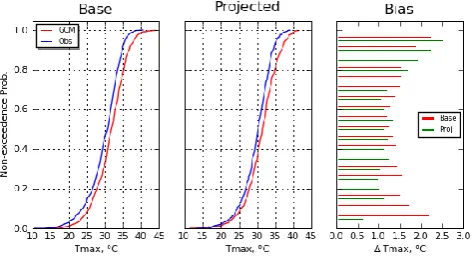
Fig. 2. Comparison of cumulative distribution functions of daily summer (JJA) maximum temperature between a GCM (NCAR CCSM3 in this case) and observations for a single grid point at 39◦N, 121◦W (cell 2 in Fig. 1). Base set is a 20 yr random sample from 1950–1999 (left panel); projected is a different 10 yr random sample from the same period (center panel), and bias (right panel) is calculated at 19 evenly spaced quantiles (0.05, 0.10, . . . , 0.95).
and since theR index is insensitive to this designation, re-sults for varying base set sizes with a fixed projected set size would be the same as those for varying projected set sizes and a fixed base set size.
3 Results and discussion
Examples of CDFs for JJA Tmax for a single grid cell for the NCAR CCSM3 GCM are illustrated in Fig. 2. For a random 20 yr base set (left panel) the GCM overestimates Tmax (relative to observations) at all quantiles, and the bias appears similar for low and high extreme values. For the 10 yr projected set (center panel), the bias appears similar to the base set, with the GCM overestimating Tmax at all quantiles. However, the bias (right panel), calculated at 19 evenly spaced quantiles (0.05, 0.10, . . . , 0.95) shows asym-metry across the quantiles. Especially noticeable is that at low quantiles, representing extreme low Tmax values, the bias for the base set is more than 1◦C greater than for the pro-jected set, while at median values the base and propro-jected set biases are closer. While this represents just one random base and projected set, it illustrates some of the potential compli-cations in assuming biases are systematic in GCM simula-tions.
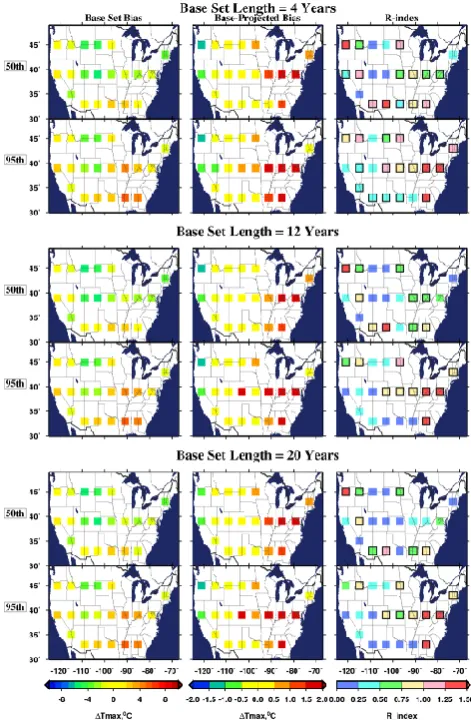
For each of 100 Monte Carlo simulations, biases relative to observations for the base and projected sets are calculated, as is the difference between the bias for the base and projected sets, and finally theR index. The results across the domain for daily JJA Tmax are illustrated in Figs. 3–5 for the GFDL model output.
a warm bias throughout the central plains, especially at the high extreme (95th percentile), well known characteristics of this version of the model (Klein et al., 2006). The magnitude of the GCM bias at specific grid cells in Fig. 3 (left panels) shows consistency for any sample of years from the late 20th century, demonstrating that there is some spatial and tempo-ral consistency in the GCM bias. This supports the concept of model deficiencies in representing detailed terrain and re-gional processes playing a role in creating the biases. Rather than the magnitude of the biases, the focus here is on deter-mining whether at each point across the domain these biases are the same between two different randomly selected sets of years.
Figure 3 also shows that the mean differences between the two sets (base and projected) of biases in GCM Tmax for both the 50th and 95th percentiles (center panels) are gener-ally smaller than the GCM bias (left panels). This is reflected in most of theR values (right panels) having a mean below one, with the worst case being with the smallest base set sam-ple (4 yr) for the extreme 95th percentile Tmax statistic. Also of note in Fig. 3 is that there is a decline in the number of grid cells whereRexceeds one between the 4 and 12 yr base set size, while little difference is evident between the 12 and 20 yr base set size. This suggests that, for daily simulations of JJA Tmax, a 12 yr base set works nearly as well as a 20 yr base set for characterizing GCM biases, both for median and extreme values, and that there is a diminishing return for us-ing larger base sets for characterizus-ing bias. The potential for using base sets of different sizes is discussed in greater detail below.
Figure 4 shows the bias and changes in bias for Tmin for the GFDL model. Of note is that the locations of high and low biases in Tmin, as with Tmax, occur in the same regions for any base set size, again supporting the concept of a time-invariant, geographically based model deficiency underlying at least a portion of the bias. It is interesting to observe in Fig. 4 that the location of greatest bias, the grid cells with the greatest change in bias, and the points withRexceeding one, are all different from Fig. 3. This suggests that the fac-tors driving biases in Tmin are distinct from those affecting Tmax, though it is beyond the scope of this effort to deter-mine the sources of the biases in GCM output. In addition, theRindex values in Fig. 4 are generally larger than in Fig. 3, with more grid cells exceeding a mean value of one for both the median and extreme at all base set sizes. This indicates that there are more grid cells in the domain where Tmin bi-ases are time dependent than for Tmax for this GCM.
[image:5.595.308.544.62.425.2]Figure 5 shows the GFDL model bias for winter precipi-tation. The left column of the biases in median and extreme daily precipitation shows one distinct pattern not as evident as in the figures of Tmax and Tmin. In particular, the biases are substantially larger for the extremes, consistent with the broad interpretation of Randall et al. (2007) that tempera-ture extremes are simulated with greater success by GCMs than precipitation extremes. As evident for Tmin (Fig. 4) the
Fig. 3. Mean bias (of 100 Monte Carlo simulations) in daily JJA Tmax for the GFDL model output for three different base set sizes (left panels), the mean difference in bias between the base and pro-jected sets (center panels), and the meanRindex value (right pan-els). Grid cells with dark outlines indicate whereRvalues are not consistently less than 1 at 95 % confidence. Projected set size is 10 yr.
Table 2. Number of grid cells (out of the 20 in the domain) with mean (of 100 Monte Carlo simulations)R >1 and, in parentheses, the number of occurrences where the 95th percentile ofRexceeds 1, for three base set sizes and two percentiles.
Tmax Tmin Pr
GCM Median Extreme Median Extreme Median Extreme
CNRM 4 yr: 2(5) 4 yr: 2(5) 4 yr: 6(15)) 4 yr: 7(10) 4 yr: 7(15) 4 yr: 8(13) 12 yr: 1(3) 12 yr: 2(5) 12yr: 5(10) 12 yr: 7(10) 12 yr: 6(11) 12 yr: 8(13) 20 yr: 1(3) 20 yr: 2(5) 20 yr: 5(8) 20 yr: 7(10) 20 yr: 5(10) 20 yr: 8(13)
GFDL 4 yr: 6(14) 4 yr: 3(9) 4 yr: 9(18) 4 yr: 5(10) 4 yr: 3(14) 4 yr: 4(8) 12 yr: 2(10) 12 yr: 3(9) 12 yr: 6(14) 12 yr: 5(10) 12 yr: 3(9) 12 yr: 4(8) 20 yr: 2(8) 20 yr: 3(9) 20 yr: 5(12) 20 yr: 5(10) 20 yr: 3(7) 20 yr: 4(8)
PCM 4 yr: 4(8) 4 yr: 5(11) 4 yr: 6(16) 4 yr: 6(12) 4 yr: 6(11) 4 yr: 6(16) 12 yr: 5(6) 12 yr: 4(9) 12 yr: 5(9) 12 yr: 3(7) 12 yr: 2(7) 12 yr: 5(10) 20 yr: 5(6) 20 yr: 3(8) 20 yr: 4(9) 20 yr: 2(7) 20 yr: 2(7) 20 yr: 5(10)
[image:6.595.47.284.299.672.2]CCSM 4 yr: 5(12) 4 yr: 2(3) 4 yr: 3(14) 4 yr: 11(18) 4 yr: 6(11) 4 yr: 3(9) 12 yr: 4(8) 12 yr: 2(3) 12 yr: 3(6) 12 yr: 11(18) 12 yr: 4(10) 12 yr: 3(9) 20 yr: 4(8) 20 yr: 2(3) 20 yr: 2(5) 20 yr: 11(18) 20 yr: 3(8) 20 yr: 3(9)
[image:6.595.307.545.302.672.2]Table 2 summarizes the right columns in Figs. 3, 4, and 5 as well as the results for the other three GCMs included in this study, to assess whether some of the same patterns ob-served for the GFDL model are shared across the four GCMs. Table 2 shows the pattern of larger base sets providing fewer occurrences ofR >1. This is more evident between 4 yr and 12 yr base sets; between 12 and 20 yr sets the results are broadly similar. However, in many cases both median and extreme values show comparable numbers ofR >1 occur-rences at all base set sizes, with the exceptions in only a few cases (e.g., GFDL median Tmax and Tmin, and PCM and CCSM median Pr). This shows that for Tmax and Pr, in the mean, bias correction would be successful in most cases us-ing base set sizes of only 4 randomly selected years. The sin-gle case where bias correction for more than half of the cells would fail, ultimately worsening the bias, is CCSM extreme Tmin, where 11 grid cells showR >1 on average. For this case, even a 20 yr base set size does not alleviate the prob-lem. This suggests that if the bias cannot be characterized with a few years of daily data, it may lack adequate time in-variance to be amenable to this form of bias correction with any number of years constituting a base set. It is interesting that this same model has the fewest number of occurrences ofR >1 for median daily Tmin, and demonstrates success-ful bias correction even with a base set of 4 yr. Thus, different processes are likely responsible for the CCSM model biases in mean and extreme daily Tmin values.
The above discussion focused on grid cells where the mean Rindex exceeded one, in which case on average the bias cor-rection degrades the skill. To examine a more stringent stan-dard, Table 2 also summarizes the number of grid cells in each case where the 95th percentileRvalues for each GCM, variable, and base set size, exceeds 1. This approximates the number of cells (outlined in Figs. 3–5) where a 95 % con-fidence thatR <1 cannot be claimed. Of the 20 grid cells analyzed in this study, as many as 18 show theR <1 hypoth-esis being rejected (CCSM extreme Tmin and GFDL median Tmin) and in other cases as few as 3 occurrences (CNRM median Tmax, CCSM extreme Tmax). While bias correction has a positive effect in the mean, the value ofRbeing below one with a high confidence (95 %) is not strongly supported, especially for Tmin and Pr.
A final observation in Table 2 of the mean number of oc-currences ofR >1 is that the GCM showing the fewest num-ber of cases varies for different variables, base set sizes, and whether median or extreme statistics are considered. Since the relative rank among GCMs is not consistent across vari-ables, it can be concluded that among the models used in this study no GCM can be broadly characterized as producing output that is more likely to benefit from statistical bias cor-rection than any other GCM. However, in the case where a specific variable is of interest, some GCMs can clearly out-perform others. For example, for maximum temperatures the CNRM model demonstrates more time invariance in biases than the other GCMs. Thus, the apparent time invariance of
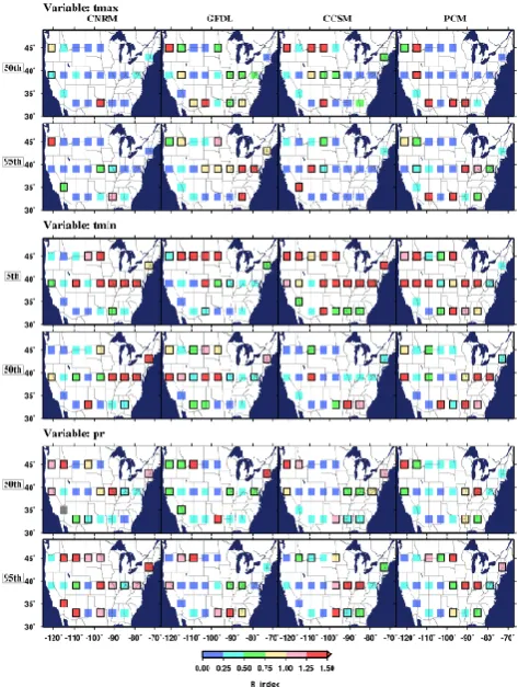
Fig. 6.R values for a 12 yr base set and a 10 yr projected set for Tmax, Tmin, and Pr for the 4 GCMs included in this study. As with Figs. 3–5, grid cells with dark outlines indicate whereRvalues are not consistently less than 1 at 95 % confidence.
biases for a specific variable and spatial domain of interest may be considered as a criterion for GCM selection when constructing ensembles, though a more comprehensive eval-uation of the effectiveness of this is reserved for future re-search.
To illustrate some of the results in Table 2, Fig. 6 shows the meanRvalues at all grid cells for a base set size of 12 yr and a projected set size of 10 yr. The most important fea-ture to note is that in most cases the grid cells where average R >1 are not the same for the different GCMs. The excep-tions to this, where more than two of the four GCMs show R >1, are the 5th percentile of minimum temperature (cells 3, 12, 15, 17), the median precipitation (cells 1, 20) and the 95th percentile precipitation (cells 6, 15, and 14). Thus, dif-ferent GCMs in general exhibit time-varying biases at differ-ent locations. This suggests that by relying on an ensemble of GCMs, a quantile mapping bias correction will be more likely on average to have a beneficial effect in removing bi-ases.
Fig. 7. Biases in seasonal statistics of daily Tmax, Tmin, and Pr based on the GFDL model from 1950–1999 at grid cell 2 (see Fig. 1). Points are biases in the median for the seasonal statistic for each year, dashed line is a 5 yr running mean, and the solid line is an 11 yr mean.
Fig. 8. Same as Fig. 7, for cell 17 (see Fig. 1).
for both the base and projected sets. With long-term per-sistence due to oceanic teleconnections producing decadal-scale variations in climate (e.g., Cayan et al., 1998), and GCMs showing improving capability to simulate similar variability (AchutaRao and Sperber, 2006), biases would be likely to show similar low frequency variability since there would not be temporal correspondence between observations and GCM simulated low frequency variations. Figures 7 and 8 show two examples of this phenomenon using the GFDL model at two locations (other models show similar behavior). It should be emphasized that because of the lack of temporal correspondence, the biases in any one year cannot be used to evaluate the GCM performance; Figs. 7 and 8 are shown only to demonstrate the low frequency variability evident in the biases. These two locations correspond to cells 2 and 17
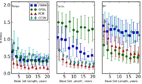
[image:8.595.116.483.304.494.2]Fig. 9. For cell number 2 (see Fig. 1),Rindex values for base set sizes from 2 to 20 yr. Points are for the meanR value for the me-dian values of the variables; the bar indicates one standard deviation centered around the point.
and Hare, 2002), and western US climate (e.g., Hidalgo and Dracup, 2003). The presence of low frequency oscillations will vary for different locations and variables. While, as ex-plained above, a time series analysis at each grid cell is not performed as part of this study, the base set size used for statistical bias correction for any region should consider the presence and frequency of regionally-important oscillations. The variation in the base set size needed to characterize the systematic bias at different locations is further complicated by the variation in the ability of GCMs to simulate certain oscillations and their teleconnections to regional precipita-tion and temperature anomalies. For the same two grid cells shown in Figs. 7 and 8, the variation inR index values for base set sizes from 2 to 20 yr is shown in Figs. 9 and 10. At both of these points bias in the median value for daily Tmax can be removed effectively, withR index values reaching a low plateau with base set sizes with fewer than 10 yr of data. The variability among GCMs is much greater for Tmin, with GFDL displaying the greatestRvalues, which remain above 1.0 even with a 20 yr base set size for cell 2. By contrast, GFDL performs best of all the GCMs at cell 17, with lowR index values achieved at 5–10 yr of base set size. Similarly, for precipitation there is a stark contrast between the GCM that shows the least ability to have its errors successfully re-moved by bias correction at the two locations. If the ability to apply bias correction successfully is to be considered as a criterion for GCM selection for a regional study, Figs. 9 and 10 demonstrate that the selection would be highly dependent on the variable and location of interest.
Recognizing that the 20 yr base set size is large relative to the size of the pool from which values are selected, this raises a concern of the degree to which the limited number of years included in this study may be affecting the results illustrated in Figs. 9 and 10, especially regarding the limited benefit of using base sets larger than about 12 yr in quan-tile mapping bias correction of daily data. While extended gridded daily observational data sets for the domain are still
Fig. 10. Same as Fig. 9, but for cell 17.
in production (Livneh et al., 2013), we obtained the data for the regions included in Figs. 9 and 10. These extended data were produced in a manner generally consistent with the original base data but includes observed data beginning in 1915, albeit with sparser station density underlying the gridded data for the earliest periods. For the GCMs included in the study, two of them (GFDL, PCM) had daily histori-cal precipitation, maximum and minimum temperature data archived for 1915–1999, which we used as our extended pe-riod of analysis. We aggregated the gridded observed precipi-tation, maximum and minimum temperature data to the same 2-degree spatial resolution for the two GCM-scale grid cells featured in Figs. 9 and 10 and repeated the analysis, with re-sults shown in Figs. 11 and 12.
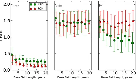
Figure 11 shows similar results to Fig. 9 for Tmax. The Rindex values for Tmin and Pr are similar to Fig. 9 for the GFDL model, but are larger for PCM, showing greater vari-ability in bias with time for PCM for the extended period analysis. However, base set sizes above about 12 yr, as with Fig. 9, appear to provide limited additional benefit in char-acterizing bias. Figure 12 is very similar to Fig. 10 for both GCMs and all 3 variables, both in the magnitude of theR values and the rate of decline in mean R value as the base set size increases. While limited in extent, this comparison between time invariance of biases using a shorter and an ex-tended base data set suggests that the analysis is relatively robust with regard to the finding that base set sizes longer than about 12 yr provide small marginal benefit.
4 Summary and conclusions
[image:9.595.309.549.61.200.2]Fig. 11. Similar to Fig. 9, but using an extended observational base period and GCM output.
between observations and GCM simulated values, and that these biases will remain the same into the future.
We performed Monte Carlo simulations, randomly select-ing years from the historic record to represent the base set, which varied in size, and a non-overlapping 10 yr projected set (drawn from a different set of years in the historical pe-riod). The biases for each Monte Carlo simulation were com-piled for a median value of each variable, and one extreme value: the 95 % (non-exceedence) precipitation, 95 % Tmax, and 5 % Tmin. For each Monte Carlo simulation, an indica-tor, here termed theR index, was computed. The R index represents the change in bias between the base and projected sets, and normalizes this by the mean bias. The mean and ap-proximate 95 % value of theRindex were calculated to as-sess the likelihood that bias correction could be successfully applied at each grid cell for each variable.
Our principal findings are:
1. In most locations, on average the GCM bias is statisti-cally the same between two different sets of years. This means a quantile-mapping bias correction on average can have a positive effect in removing a portion of the GCM bias.
2. For characterizing daily GCM output, our findings indi-cate variability in the number of years required to char-acterize bias for different GCMs and variables. On av-erage a base set with as few as 4 randomly-selected years is often adequate to characterize the biases in daily GCM precipitation and temperature, at both median and extreme values. A base set of 12 yr provided improve-ment in the number of grid cells where high confidence in successful bias correction could be claimed.
[image:10.595.50.287.62.199.2]3. For most variables and GCMs the characterization of the bias shows little improvement with base set sizes larger than about 10 yr. In a few cases the variability in bias between different sets of years is high enough that even a 20 yr base set size cannot provide the necessary
Fig. 12. Similar to Fig. 10, but using an extended observational base period and GCM output.
time invariance between sets of years to allow success-ful bias correction with quantile mapping.
4. When considering consecutive rather than randomly se-lected years, the GCM biases exhibit low frequency variability similar to observations, and the selected base period must be long enough to remove their effect. 5. At any location, the biases in the base and projected
sets of years for a particular variable were fairly con-sistent for any given GCM, regardless of base set size. This reflects that there are geographical manifestations to some of the GCM shortcomings that cause bias, such as the inadequate topography represented at coarse res-olutions. There are differences between the magnitude of biases at the mean and extreme values (especially for precipitation), but the differences in the biases between the base and projected sets of years are comparable for both mean and extreme values.
Since this study only examined the stationarity in time of daily GCM biases, those at longer timescales are not ex-plicitly addressed. However, Maurer et al. (2010) show that a quantile mapping bias correction of daily data can result in the removal of most biases in monthly GCM output. In another study, Coats et al. (2013), with details in Coats et al. (2010), found that quantile mapping of precipitation at the daily timescale resulted in monthly and annual distribu-tions in remarkably good agreement with observadistribu-tions. This suggests that by bias correcting at a daily scale the biases at longer timescales may also be accommodated.
Future work will extend this analysis for the new model formulations producing climate simulations for the IPCC Fifth Assessment for a larger ensemble and a longer observa-tional period. This will allow the testing of model simulations for a longer observational period including the most recent decade, when large-scale warming has accelerated, provid-ing more extreme cases for the above tests. Biases and their time invariance will also be investigated at scales finer than the 2◦resolution used in this study, reflecting both the finer resolution of the new GCMs and the latest implementations of quantile mapping bias correction at finer scales. In addi-tion, new daily observational data sets of close to 100 yr in length (e.g., Casola et al., 2009) will allow more intensive investigation of GCM biases by facilitating compositing on different conditions such as regional climate or oscillation phase.
Acknowledgements. This research was supported in part by the California Energy Commission Public Interest Energy Research (PIER) Program. During the development of the majority of this work, T. Das was working as a scientist at Scripps Institution of Oceanography. The CALFED Bay-Delta program post-doctoral fellowship provided partial support for T. Das. The authors are grateful for the thoughtful and constructive comments of the reviewers, whose feedback substantially improved our methods and interpretation of results.
Edited by: L. Samaniego
References
Abatzoglou, J. T. and Brown, T. J.: A comparison of statistical downscaling methods suited for wildfire applications, Int. J. Cli-matol., 32, 772–780, doi:10.1002/joc.2312, 2012.
AchutaRao, K. M. and Sperber, K. R.: ENSO Simulation in Cou-pled Ocean-Atmosphere Models: Are the Current Models Bet-ter?, Clim. Dynam., 27, 1–15, doi:10.1007/s00382-006-0119-7, 2006.
Ballester, J., Giorgi, F., and Rodo, X.: Changes in European tem-perature extremes can be predicted from changes in PDF central statistics, Climatic Change, 98, 277–284, doi:10.1007/s10584-009-9758-0, 2010.
Bo´e, J., Terray, L., Habets, F., and Martin, E.: Statistical and dynamical downscaling of the Seine basin climate for
hydro-meteorological studies, Int. J. Climatol., 27, 1643–1655, doi:10.1002/joc.1602, 2007.
B¨urger, G., Murdock, T. Q., Werner, A. T., Sobie, S. R., and Cannon, A. J.: Downscaling Extremes – An Intercomparison of Multiple Statistical Methods for Present Climate, J. Climate, 25, 4366– 4388, doi:10.1175/jcli-d-11-00408.1, 2012.
Buser, C. M., Kunsch, H. R., Luthi, D., Wild, M., and Schar, C.: Bayesian multi-model projection of climate: bias assump-tions and interannual variability, Clim. Dynam., 33, 849–868, doi:10.1007/s00382-009-0588-6, 2009.
Carter, T. R., Jones, R. N., Lu, X., Bhadwal, S., Conde, C., Mearns, L. O., O’Neill, B. C., Rounsevell, M. D. A., and Zurek, M. B.: New Assessment Methods and the Characterisation of Fu-ture Conditions. Climate Change 2007: Impacts, Adaptation and Vulnerability. Contribution of Working Group II to the Fourth Assessment Report of the Intergovernmental Panel on Climate Change, in, edited by: Parry, M. L., Canziani, O. F., Palutikof, J. P., van der Linden, P. J., and Hanson, C. E., Cambridge Univer-sity Press, Cambridge, UK, 133–171, 2007.
Casola, J. H., Cuo, L., Livneh, B., Lettenmaier, D. P., Stoelinga, M. T., Mote, P. W., and Wallace, J. M.: Assessing the Impacts of Global Warming on Snowpack in the Washington Cascades*, J. Climate, 22, 2758–2772, doi:10.1175/2008jcli2612.1, 2009. Cayan, D. R., Dettinger, M. D., Diaz, H. F., and Graham,
N. E.: Decadal Variability of Precipitation over Western North America, J. Climate, 11, 3148–3166, doi:10.1175/1520-0442(1998)011<3148:DVOPOW>2.0.CO;2, 1998.
Chen, C., Haerter, J. O., Hagemann, S., and Piani, C.: On the con-tribution of statistical bias correction to the uncertainty in the projected hydrological cycle, Geophys. Res. Lett., 38, L20403, doi:10.1029/2011gl049318, 2011.
Christensen, J. H., Hewitson, B., Busuioc, A., Chen, A., Gao, X., Held, I., Jones, R., Kolli, R. K., Kwon, W.-T., Laprise, R., Maga˜na Rueda, V., Mearns, L., Men´endez, C. G., R¨ais¨anen, J., Rinke, A., Sarr, A., and Whetton, P.: Regional climate projec-tions, in: Climate Change 2007: The Physical Science Basis. Contribution of Working Group I to the Fourth Assessment Re-port of the Intergovernmental Panel on Climate Change, edited by: Solomon, S., Qin, D., Manning, M., Chen, Z., Marquis, M., Averyt, K. B., Tignor, M., and Miller, H. L., Cambridge Uni-versity Press, Cambridge, United Kingdom and New York, NY, USA, 2007.
Christensen, J. H., Boberg, F., Christensen, O. B., and Lucas-Picher, P.: On the need for bias correction of regional climate change projections of temperature and precipitation, Geophys. Res. Lett., 35, L20709, doi:10.1029/2008gl035694, 2008. Coats, R., Reuter, J., Dettinger, M., Riverson, J., Sahoo, G.,
Schladow, G., Wolfe, B., and Costa-Cabral, M.: The effects of climate change on Lake Tahoe in the 21st century: Meteorol-ogy, hydrolMeteorol-ogy, loading and lake response, Pacific Southwest Re-search Station, Tahoe Environmental Science Center, Incline Vil-lage NV, USA, 208, 2010.
Coats, R., Costa-Cabral, M., Riverson, J., Reuter, J., Sahoo, G., Schladow, G., and Wolfe, B.: Projected 21st century trends in hydroclimatology of the Tahoe basin, Climatic Change, 116, 51– 69, doi:10.1007/s10584-012-0425-5, 2013.
Delworth, T. L., Broccoli, A. J., Rosati, A., Stouffer, R. J., Balaji, V., Beesley, J. A., Cooke, W. F., Dixon, K. W., Dunne, J., Dunne, K. A., Durachta, J. W., Findell, K. L., Ginoux, P., Gnanadesikan, A., Gordon, C. T., Griffies, S. M., Gudgel, R., Harrison, M. J., Held, I. M., Hemler, R. S., Horowitz, L. W., Klein, S. A., Knutson, T. R., Kushner, P. J., Langenhorst, A. R., Lee, H.-C., Lin, S.-J., Lu, J., Malyshev, S. L., Milly, P. C. D., Ramaswamy, V., Russell, J., Schwarzkopf, M. D., Shevliakova, E., Sirutis, J. J., Spelman, M. J., Stern, W. F., Winton, M., Wittenberg, A. T., Wyman, B., Zeng, F., and Zhang, R.: GFDL’s CM2 global coupled climate models – Part 1: Formulation and simulation characteristics, J. Climate, 19, 643–674, 2006.
Ehret, U., Zehe, E., Wulfmeyer, V., Warrach-Sagi, K., and Liebert, J.: HESS Opinions “Should we apply bias correction to global and regional climate model data?”, Hydrol. Earth Syst. Sci., 16, 3391–3404, doi:10.5194/hess-16-3391-2012, 2012.
Fowler, H. J., Blenkinsop, S., and Tebaldi, C.: Linking climate change modelling to impacts studies: recent advances in down-scaling techniques for hydrological modelling, Int. J. Climatol., 27, 1547–1578, doi:10.1002/joc.1556, 2007.
Frich, P., Alexander, L. V., Della-Marta, P., Gleason, B., Haylock, M., Klein Tank, A. M. G., and Peterson, T. C.: Observed Coher-ent changes in climatic extremes during the second half of the twentieth century, Clim. Res., 19, 193–212, 2002.
Haerter, J. O., Hagemann, S., Moseley, C., and Piani, C.: Cli-mate model bias correction and the role of timescales, Hy-drol. Earth Syst. Sci., 15, 1065–1079, doi:10.5194/hess-15-1065-2011, 2011.
Hall, A., Qu, X., and Neelin, J. D.: Improving predictions of sum-mer climate change in the United States, Geophys. Res. Lett., 35, L01702, doi:10.1029/2007GL032012, 2008.
Hawkins, E. and Sutton, R.: The Potential to Narrow Uncertainty in Regional Climate Predictions, B. Am. Meteorol. Soc., 90, 1095– 1107, doi:10.1175/2009BAMS2607.1, 2009.
Hewitson, B.: Developing perturbations for climate change im-pact assessments, EOS T. Am. Geophys. Un., 84, 337–341, doi:10.1029/2003EO350001, 2003.
Hidalgo, H. G. and Dracup, J. A.: ENSO and PDO Ef-fects on Hydroclimatic Variations of the Upper Colorado River Basin, J. Hydrometeorol., 4, 5–23, doi:10.1175/1525-7541(2003)004<0005:eapeoh>2.0.co;2, 2003.
Ines, A. V. M. and Hansen, J. W.: Bias correction of daily GCM rainfall for crop simulation studies, Agr. Forest Meteorol., 138, 44–53, 2006.
Karl, T. R., Melillo, J. M., and Peterson, D. H.: Global climate change impacts in the United States, Cambridge University Press, New York, 192 pp., 2009.
Kiehl, J. T., Hack, J. J., Bonan, G. B., Boville, B. B., Williamson, D. L., and Rasch, P. J.: The National Center for Atmospheric Re-search Community Climate Model: CCM3, J. Climate, 11, 1131– 1149, 1998.
Klein, S. A., Jiang, X., Boyle, J., Malyshev, S., and Xie, S.: Di-agnosis of the summertime warm and dry bias over the U.S. Southern Great Plains in the GFDL climate model using a weather forecasting approach, Geophys. Res. Lett., 33, L18805, doi:10.1029/2006gl027567, 2006.
Knutti, R., Allen, M. R., Friedlingstein, P., Gregory, J. M., Hegerl, G. C., Meehl, G. A., Meinshausen, M., Murphy, J. M., Plattner, G. K., Raper, S. C. B., Stocker, T. F., Stott, P. A., Teng, H., and
Wigley, T. M. L.: A review of uncertainties in global temperature projections over the twenty-first century, J. Climate, 21, 2651– 2663, doi:10.1175/2007jcli2119.1, 2008.
Lafon, T., Dadson, S., Buys, G., and Prudhomme, C.: Bias cor-rection of daily precipitation simulated by a regional climate model: a comparison of methods, Int. J. Climatol., 33, 1367– 1381, doi:10.1002/joc.3518, 2012.
Li, H., Sheffield, J., and Wood, E. F.: Bias correction of monthly precipitation and temperature fields from Intergovern-mental Panel on Climate Change AR4 models using equidis-tant quantile matching, J. Geophys. Res., 115, D10101, doi:10.1029/2009jd012882, 2010.
Livneh, B., Rosenberg, E. A., Lin, C., Nijssen, B., Mishra, V., An-dreadis, K., Maurer, E. P., and Lettenmaier, D. P.: A Long-term hydrologically based dataset of land surface fluxes and states for the conterminous U.S.: Update and extensions, 25th Conference on Climate Variability and Change, 93rd American Meteorolog-ical Society Annual Meeting, Austin, TX, USA, Paper 6A.3, 2013.
Macadam, I., Pitman, A. J., Whetton, P. H., and Abramowitz, G.: Ranking climate models by performance using actual values and anomalies: Implications for climate change impact assessments, Geophys. Res. Lett., 37, L16704, doi:10.1029/2010gl043877, 2010.
Mantua, N. J. and Hare, S. R.: The Pacific Decadal Oscillation, J. Oceanogr., 58, 35–44, 2002.
Maraun, D.: Nonstationarities of regional climate model biases in European seasonal mean temperature and precipitation sums, Geophys. Res. Lett., 39, L06706, doi:10.1029/2012gl051210, 2012.
Maraun, D., Wetterhall, F., Ireson, A. M., Chandler, R. E., Kendon, E. J., Widmann, M., Brienen, S., Rust, H. W., Sauter, T., The-meßl, M., Venema, V. K. C., Chun, K. P., Goodess, C. M., Jones, R. G., Onof, C., Vrac, M., and Thiele-Eich, I.: Precipi-tation downscaling under climate change: Recent developments to bridge the gap between dynamical models and the end user, Rev. Geophys., 48, RG3003, doi:10.1029/2009rg000314, 2010. Masson, D. and Knutti, R.: Spatial-Scale Dependence of Climate
Model Performance in the CMIP3 Ensemble, J. Climate, 24, 2680–2692, doi:10.1175/2011jcli3513.1, 2011.
Maurer, E. P., Wood, A. W., Adam, J. C., Lettenmaier, D. P., and Nijssen, B.: A long-term hydrologically-based data set of land surface fluxes and states for the conterminous United States, J. Climate, 15, 3237–3251, 2002.
Maurer, E. P., Hidalgo, H. G., Das, T., Dettinger, M. D., and Cayan, D. R.: The utility of daily large-scale climate data in the assess-ment of climate change impacts on daily streamflow in Califor-nia, Hydrol. Earth Syst. Sci., 14, 1125–1138, doi:10.5194/hess-14-1125-2010, 2010.
Meehl, G. A., Covey, C., Delworth, T., Latif, M., McAvaney, B., Mitchell, J. F. B., Stouffer, R. J., and Taylor, K. E.: The WCRP CMIP3 multimodel dataset: A new era in climate change re-search, B. Am. Meteorol. Soc., 88, 1383–1394, 2007.
Panofsky, H. A. and Brier, G. W.: Some Applications of Statistics to Meteorology, The Pennsylvania State University, University Park, PA, USA, 224 pp., 1968.
doi:10.1007/s00704-009-0134-9, 2010.
Pierce, D. W., Das, T., Cayan, D., Maurer, E. P., Bao, Y., Kanamitsu, M., Yoshimura, K., Snyder, M. A., Sloan, L. C., Franco, G., and Tyree, M.: Probabilistic estimates of future changes in Califor-nia temperature and precipitation using statistical and dynamical downscaling, Clim. Dynam., 40, 839–856, doi:10.1007/s00382-012-1337-9, 2013.
Pyke, C. B.: Some meteorological aspects of the seasonal distribu-tion of precipitadistribu-tion in the western United States and Baja Cali-fornia, University of California Water Resources Center Contri-bution 139, Berkeley, CA, 205, 1972.
Randall, D. A., Wood, R. A., Bony, S., Colman, R., Fichefet, T., Fyfe, J., Kattsov, V., Pitman, A., Shukla, J., Srinivasan, J., Sumi, A., Stouffer, R. J., and Taylor, K. E.: Climate models and their evaluation, in: Climate Change 2007: The Physical Science Ba-sis. Contribution of Working Group I to the Fourth Assessment Report of the Intergovernmental Panel on Climate Change, edited by: Solomon, S., Qin, D., Manning, M., Chen, Z., Marquis, M., Averyt, K. B., Tignor, M., and Miller, H. L., Cambridge Univer-sity Press, Cambridge, UK, 591–648, 2007.
Salas-M´elia, D., Chauvin, F., D´equ´e, M., Douville, H., Gueremy, J. F., Marquet, P., Planton, S., Royer , J. F., and Tyteca, S.: Description and validation of the CNRM-CM3 global coupled model, CNRM working note 103, Centre National de Recherches M´et´eorologiques, M´et´eo-France, Toulouse, France, 36 pp., 2005. Sun, Y., Solomon, S., Dai, A., and Portmann, R. W.: How Often Does It Rain?, J. Climate, 19, 916–934, doi:10.1175/jcli3672.1, 2006.
Tebaldi, C., Hayhoe, K., Arblaster, J. M., and Meehl, G. A.: An intercomparison of model-simulated historical and future changes in extreme events, Climatic Change, 79, 185–211, doi:10.1007/s10584-006-9051-4, 2006.
Themeßl, M., Gobiet, A., and Heinrich, G.: Empirical-statistical downscaling and error correction of regional climate models and its impact on the climate change signal, Climatic Change, 112, 449–468, doi:10.1007/s10584-011-0224-4, 2012.
Thrasher, B., Maurer, E. P., McKellar, C., and Duffy, P. B.: Techni-cal Note: Bias correcting climate model simulated daily temper-ature extremes with quantile mapping, Hydrol. Earth Syst. Sci., 16, 3309–3314, doi:10.5194/hess-16-3309-2012, 2012. Tryhorn, L. and DeGaetano, A.: A comparison of techniques for
downscaling extreme precipitation over the Northeastern United States, Int. J. Climatol., 31, 1975–1989, doi:10.1002/joc.2208, 2011.
Vicuna, S., Dracup, J. A., Lund, J. R., Dale, L. L., and Maurer, E. P.: Basin-scale water system operations with uncertain future cli-mate conditions: Methodology and case studies, Water Resour. Res., 46, W04505, doi:10.1029/2009WR007838, 2010. Washington, W. M., Weatherly, J. W., Meehl, G. A., Semtner, A. J.,
Bettge, T. W., Craig, A. P., Strand, W. G., Arblaster, J., Wayland, V. B., James, R., and Zhang, Y.: Parallel climate model (PCM) control and transient simulations, Clim. Dynam., 16, 755–774, 2000.
Wehner, M.: Sources of uncertainty in the extreme value statistics of climate data, Extremes, 13, 205–217, doi:10.1007/s10687-010-0105-7, 2010.
Wood, A. W., Leung, L. R., Sridhar, V., and Lettenmaier, D. P.: Hy-drologic implications of dynamical and statistical approaches to downscaling climate model outputs, Climatic Change, 62, 189– 216, 2004.