www.hydrol-earth-syst-sci.net/16/4101/2012/ doi:10.5194/hess-16-4101-2012
© Author(s) 2012. CC Attribution 3.0 License.
Earth System
Sciences
Joint statistical correction of clutters, spokes and beam height for a
radar derived precipitation climatology in southern Germany
A. Wagner1,2,*, J. Seltmann1, and H. Kunstmann2,3
1German Met. Service (DWD), Meteor. Observatory, Hohenpeissenberg, Germany
2University of Augsburg, Institute for Geography, Regional Climate and Hydrology, Augsburg, Germany 3Karlsruhe Institute of Technology, Institute for Meteorology and Climate Research IMK-IFU,
Garmisch-Partenkirchen, Germany
*now at: HYDRON GmbH, Karlsruhe, Germany
Correspondence to: A. Wagner ([email protected])
Received: 19 March 2012 – Published in Hydrol. Earth Syst. Sci. Discuss.: 13 April 2012 Revised: 28 September 2012 – Accepted: 30 September 2012 – Published: 7 November 2012
Abstract. First results of radar derived climatology have emerged over the last years, as datasets of appropriate extent are becoming available. Usually, these statistics are based on time series lasting up to ten years as continuous storage of radar data was often not achieved before. This kind of clima-tology demands a high level of data quality. Small deviations or minor systematic under- or overestimations in single radar images become a major cause of error in statistical analysis. Extensive corrections of radar data are a crucial prerequisite for radar derived climatology. We present a new statistical post-correction scheme based on a climatological analysis of seven years of radar data of the Munich weather radar (2000– 2006) operated by DWD (German Weather Service). Origi-nal radar products are used subject only to corrections within the signal processor without any further corrections on sin-gle radar images. The aim of this statistical correction is to make up for the average systematic errors caused by clutter, propagation, or measuring effects but to conserve small-scale natural variations in space.
The statistical correction is based on a thorough analysis of the different causes of possible errors for the Munich weather radar. This analysis revealed the following basic effects: the decrease of rain amount as a function of height and distance from the radar, clutter effects such as clutter remnants after filtering, holes by eliminated clutter or shading effects from obstacles near the radar, visible as spokes, as well as the in-fluence of the bright band. The correction algorithm is corre-spondingly based on these results. It consists of three mod-ules. The first one is an altitude correction which minimises
measuring effects. The second module corrects clutter effects and disturbances and the third one realises a mean adjustment to selected rain gauges. Two different sets of radar products are used. The statistical analysis as well as module 1 and module 2 of the correction algorithm are based on frequen-cies of the six reflectivity levels within the so-called PX prod-uct. For correction module 3 and for the validation of the correction algorithm, rain amounts are calculated from the 8-bit so-called DX product. The correction algorithm is created to post-correct climatological or statistical analysis of radar data with a temporal resolution larger than one year. The correction algorithm is used for frequencies of occurrence of radar reflectivities which enables its application even for radar products such as DWD’s cell-tracking-product CON-RAD.
1 Introduction
The spatiotemporal distribution of precipitation is the cen-tral meteorological variable regarding hydrological analyses. Its measurement is very demanding at the same time. Satel-lite data is still not precise enough whereas its areal cover-age is excellent. Point measurements suffer from areal ex-trapolation errors particularly in cases of precipitation with high variations in space. Weather radar data offers a good compromise between areal rain structure and measuring ac-curacy. But this is only true if a number of influencing factors are taken into account, which usually lead to certain correc-tions that have to be applied before radar data is processed further (Holleman, 2007). Among the huge number of influ-encing factors the conversion of radar reflectivity into rain rate (e.g., Z/R-relationship) is one of the biggest challenges, as it is heavily dependent on drop size distributions of rain which is usually highly variable in space and time. The melt-ing layer (bright band) with higher radar reflectivities at a certain altitude and lower reflectivities in the snow is an-other major concern in the correction of radar data as its influence affects huge parts of the radar image and can ex-ceed the influence of the Z/R-relationship especially in the temperate zone in spring and autumn (e.g., Fabry and Za-wadzki, 1995; Franco et al., 2006; Haase et al., 2005; Joss and Lee, 1995; Kitchen et al., 1994; Koistinen, 1991; Kra-jewski et al., 2010; S´anchez-Diezma et al., 2000; Vignal et al., 1999). However, no bright band correction is operational at DWD so far. Differences in reflectivities at different al-titudes are often naturally induced. Besides the bright band influence and the transition from snow to rain, the low verti-cal extension of clouds may result in partial beam-filling or overshooting, and the beam filling inhomogeneity increases with beam width. Attenuation behind strong convective cells, non-meteorological echoes like insects, birds, planes, ships and windmills or shading effects behind buildings and moun-tains are further sources of errors in radar data which have to be paid attention to.
For the analysis of single radar images a thorough usage of correction algorithms usually leads to a good data basis for areal precipitation. Little deviations or small systematic underestimations or overestimations are negligible. But for statistical analysis of a larger number of radar measurements these deviations may become a major cause of error. Sev-eral ways to deal with this problem are feasible. Koistinen et al. (2008) and Overeem et al. (2009), for example, make an effort in correcting single radar images. An alternative ap-proach, followed in this study, is to solely rely on statistical corrections. Original radar products are used including only corrections within the signal processor (Doppler filtering, speckle remover, thresholding for noise (log), signal qual-ity (spectral width with SNR) and clutter correction) with-out any further corrections on single radar images. The result of the statistical analysis from radar images is corrected sta-tistically. The aim of this statistical correction is to remove
errors caused by insufficiently corrected clutter, influences of shading-effects resulting in spokes in radar images or the deviations caused by increasing beam height and beam width with distance from the radar, but to conserve small-scale nat-ural variations in space. Although these errors are highly variable for single radar images, the net effect of these er-rors may be statistically addressed. The correction algorithm is empirical as very often the reason for a spatial variation is a mixture of several determining factors which cannot be separated. Nevertheless, a thorough analysis of the different causes of deviations and their behaviour in space and time is essential to establish a reliable correction algorithm.
Section 2 gives a brief overview of the investigation area and the different data types used. The main theme and the used method are described in Sect. 3. In Sect. 4 the data basis of the statistical correction is analysed. Deviations in radar images are classified, examined and discussed. These results are the basis for the way the statistical corrections are estab-lished. These are described in Sect. 5. Section 6 includes a validation of the correction algorithm using rain gauges.
2 Data
Fig. 1. Mean altitudes of the near-surface precipitation scan of the Munich Weather Radar (2000–2006). Overplotted by locations of the rain gauges used for comparing rain amounts.
Additionally, the range of the Alps leads to clutter and shad-ing effects in the southern part of the radar image.
Two different radar products based on the precipitation scan were used for this analysis. The so-called PX product with six reflectivity levels (see Table 1) and a spatial resolu-tion of 1×1 km2has the longest time-series starting in 2000. It includes a threshold for noise. The lower limit of reflec-tivity level 1 is 7 dBZ in summer and 1 dBZ in winter. This radar product for the years 2000 to 2006 is the basis for the analysis of disturbances within the radar image as well as for the development of the correction algorithms. The availabil-ity of this product for the Munich weather radar is between 75 % and 95 % per year. The inner 100 km from the radar site are analysed, which results in a total of 2.4×1010 pixel-measurements as a profound basis for a statistical analysis.
The second radar product used is the DX product with 256 classes from−31.5 dBZ to 95.5 dBZ and a resolution of 0.5 dBZ. For this analysis the reflectivity range has been lim-ited. It ranges from 1 dBZ (noise) to 60 dBZ (hail). Its origi-nal resolution is 1◦in azimuth-direction and 1 km in range.
This product is also only based on the near-surface precip-itation scan every 5 min, just as the PX product. It is ideal for quantitative purposes and is, therefore, used for adjustment of radar data to rain gauges and for means of validation. It has continuously been stored since 2004 for the Munich weather radar and its availability is about 85 % until 2006 and after-wards between 95 % and 98 %.
91 rain gauges in the vicinity of the Munich weather radar with reliable time-series of daily precipitation measurements were available for the comparison with the radar DX prod-uct. Tipping-buckets as well as rain collectors from DWD are used both quality controlled according to official qual-ity insurance standards. The temporal resolution was daily.
The original database was 140 rain gauges. Only 91 rain gauges cover the total time range from 2004 to 2009, showed only few missing-values for longer times and accomplished the following additional quality controls. The rain gauges were manually quality controlled for any bias including limit exceedance of daily, monthly and annually mean values as well as intercompared to time series of adjacent rain gauges. Three groups of rain gauges were established: the first group consists of 33 gauges within a distance from 30 to 60 km from the radar site representing the area of the most reli-able radar measurements; the second one are 76 rain gauges within the whole radar coverage excluding those which are situated in regions of radar-pixel interpolation like parts of the alpine region or the city of Munich; the third group in-cludes all 91 rain gauges. The locations of the rain gauges are plotted in Fig. 1.
3 Method
Both the analysis of corrupted pixels within radar images of the Munich weather radar and the corrections that are derived from these analyses, are based on the frequency of occur-rence of radar reflectivities for each reflectivity level of the PX product. The reflectivity levels 1, 3 and 5 identified to light, moderate and heavy rain are presented.
Especially for extreme rainfall, climatology of radar data seems very promising (Overeem et al., 2010; Pedersen et al., 2008; Rudolph et al., 2011; Wagner et al., 2006). We also focus on the development of a correction algorithm espe-cially for moderate and heavy precipitation with a profound database. Particularly, CONRAD-data (Convection in Radar Products) that is based on the PX product shall be corrected. For light and moderate rain the database is large enough to rely on these results, whereas for heavy precipitation the database is too scarce to only rely on these results. So also light rain and moderate rain is analysed. The aim is to pos-sibly transfer from the findings of light and moderate rain to heavy precipitation or to support the results of heavy precip-itation.
A statistical correction aims at improving the quality on average. The advantage of such a statistical correction is that no single disturbance variables, but only their overall impact have to be taken into account. The disadvantage is closely related: assumptions are necessary, whether a certain pattern is a measuring bias or naturally induced as its source is often not distinctively or a mixture of different reasons.
Table 1. Reflectivity levels of the PX product.
Reflectivity (dBZ) 1 (7)–18.9 19–27.9 28–36.9 37–45.9 46–54.9 ≥55
Rain rate (mm h−1) 0.1–1 1–3 3–9 9–27 27–80 >80
Class 1 2 3 4 5 6
regarded as bias. Variations within such a ring are regarded as naturally induced. Certain geographical characteristics re-sulting in different meteorological situations with different rain amounts are not specifically taken into account but re-main in the database. Conversely, abrupt variations of fre-quencies of occurrence in space indicate errors in data basis, as does a general increase or decrease in these frequencies with height or distance from the radar.
The first step of the analysis is to identify pixel groups within the radar image that are obviously affected by the same type of clutter. Three different types of clutter were classified: the “city clutter” of Munich caused by obstacles within a distance of 40 km to the south of the radar site, “mountain clutter” of the Alps in the South at distances of over 70 km from the radar site and “spokes” originating from obstacles near the radar. Basically, each type of clutter or dis-turbance can be identified as long as its appearance is statis-tically significant. Figure 2 gives an overview of corrupted and uncorrupted radar pixels for reflectivity level 1. The red colour represents pixels which are affected by clutter or clut-ter correction and the orange colour indicates spokes. The city clutter and the mountain clutter can easily be separated because of the underlying landscape. For these two clutter types, a certain area including corrupted pixels of the same source is visually defined, where uncorrupted pixels form the majority of pixels. The blue colour in Fig. 2 indicates the area of mountain clutter. Pixels in this area should have compara-ble beam heights and distances from the radar. Corrupted and uncorrupted pixels within these areas have to be separated. This separation has only been made once and includes man-ual work. For each area of correction, thresholds of frequen-cies of occurrence are used to separate those pixels which are obviously corrupted from the rest. Additionally, a buffer of 2 km is established around the corrupted pixels to mark those pixels which are likely to be influenced by clutter. For the residual pixels a histogram of frequencies of occurrence is established. The uncorrupted pixels (comparison group) show comparable frequencies of occurrence and, therefore, form a distinctive peak in the histogram. Pixels which differ from this distribution can be separated manually if the pre-selection of uncorrupted pixels was difficult. As a last step, the final separation is realised by the analysis of an empiri-cal distribution of frequencies of occurrence, where its 95 % interval marks the range of uncorrupted pixels. As reflectiv-ity level 1 shows the highest amount of corrupted pixels, the classification for all levels is based on level 1.
Fig. 2. Overview of clutter and disturbances for reflectivity level 1 of the Munich weather radar including clutter pixels (red), spokes (yellow) and the comparison area of uncorrupted radar pixels for the mountain clutter (blue).
For the spokes, the separation of corrupted and uncor-rupted pixels is similar, but all pixels within one azimuth (1◦resolution) are treated jointly. First, for each azimuth the
median of all pixels except those affected by city clutter or mountain clutter, is calculated. Using thresholds, the obvious spokes can be separated from uncorrupted pixels. The tran-sition from uncorrupted pixels to a spoke forms a distinctive gradient, so the extension of one spoke can be determined by comparing the median of adjacent azimuths. If the me-dian differs more than 10 % this usually is an indication for the transition from uncorrupted to corrupted azimuth angles. This can be checked visually.
The uncorrupted radar pixels were analysed for measur-ing effects, as beam height and beam width increase with distance from the radar. Pixels were classified according to their beam height. All 5-min radar images are used to cal-culate the frequency of occurrence of each reflectivity level for every radar pixel in a certain altitude class (one class per 100 m). Then, the median for each altitude class and level is calculated and plotted against height. In this way, the mean decrease in frequency of occurrences with height is further analysed.
[image:4.595.332.519.130.338.2]is compared to the median of the corresponding frequency of occurrence of adjacent undisturbed radar pixels (comparison group). In this way, these patterns are analysed with regard to their situation, the circumstances they depend on and the reason for their occurrence.
According to the results of the statistical analysis of the radar images some systematic behaviour was deduced. Two of the three modules of the correction algorithm are closely based on these findings. The first module is an “altitude cor-rection” based on a linear regression model. The second module is the “correction of clutter effects” using derived correction factors or interpolation methods.
The DX radar product is used for the comparison of rain amounts from rain gauges to rain amounts from correspond-ing radar pixels. This has two objectives: first, a mean bias correction factor is derived from this comparison to adjust mean annual rain amounts from radar data to rain amounts from rain gauges. This “adjustment” represents the third module of the correction algorithm. Secondly, the compar-ison with data from rain gauges acts as a quality check for the correction algorithm with an independent data basis (cali-bration/validation). A perfect match of precipitation amounts derived from radar and precipitation from rain gauges is im-probable due to different measuring effects. A radar mea-sures at a different height and samples a larger volume com-pared to a rain gauge. Regarding convective rain events the representativeness of a point measurement is often only a few metres. Thus, representativeness errors result. So, not the characteristics of the whole time-series of precipitation are compared, but only the integral mean annual amount of rain. It is more important that the average proportion of the rain amounts of rain gauges and their corresponding radar pixels close to the radar is equal to the average proportion of the rain amounts of rain gauges and their corresponding radar pixels at greater distances from the radar than their absolute magnitude is. The calculation of an adjustment factor with a higher temporal resolution may additionally improve the use-fulness of this correction. However, in that case the transfer of, for example, a daily correction factor from one year to the next is problematic. A central aim of the adjustment here is to correct the side-effect of the altitude correction. The altitude correction equalises the frequencies of occurrence at differ-ent ranges, but at the same time it overestimates the measured frequencies of occurrence and rain rates (see Sect. 5.1). This adjustment is only useful on an annual basis at least for light and moderate rain. So the adjustment factor and the altitude correction are closely related.
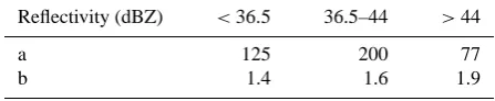
A three-part Z/R-relationship (cf. Table 2) is used to cal-culate rain rate from radar reflectivities of the DX product (Bartels et al., 2004). This relationship considers different drop size spectra of light, moderate and heavy rain by using three different Z/R-relationships according to radar reflectiv-ity.
[image:5.595.315.539.94.140.2]Two periods of time were defined for the comparison of rain amounts from radar data and rain gauges. The first
Table 2. Three-part Z/R-relationship used to calculate rain rate from DX radar products.
Reflectivity (dBZ) <36.5 36.5–44 >44
a 125 200 77
b 1.4 1.6 1.9
period from 2004 to 2006 is the period of calibration and adjustment, 2007 to 2009 is the period of validation. The pre-requisite for a transfer of the corrections from one period to the next is that either no crucial changes in electronic cal-ibration or scan strategy were implemented or the changes are analysed on the basis of at least one year of radar data. In 2004, a new signal processor was installed and the beam elevation angles were optimised in 2006. As a consequence, the correction of spokes had to be updated.
4 Analysis of disturbances in radar images
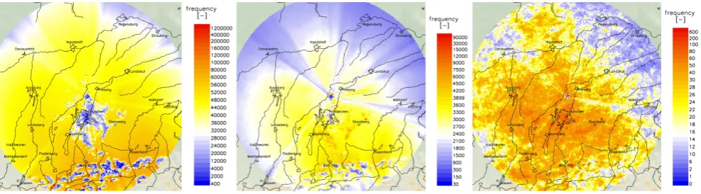
Figure 3 gives an overview of the frequency of occurrence of radar reflectivities for level 1 (light rain), level 3 (moderate rain) and level 5 (heavy rain). The three main types of clutter and disturbances (city clutter, mountain clutter and spokes) become obvious within the vicinity of the Munich weather radar. A comparison of these three radar images reveals con-spicuous differences of the values of the clutter disturbances. The “uncorrupted” radar pixels show a significant decrease of the frequency of radar reflectivities with height of the radar pixel above ground level for all radar reflectivities (variations with height).
4.1 Variations with height
Fig. 3. Uncorrected frequencies of occurrence of radar reflectivity level 1 (left), level 3 (middle) and level 5 (right) of the Munich weather radar from 2000–2006 (PX data). The scale is 200×200 km2.
profiles for the cell stages of cumulonimbus clouds. For most stages reflectivities between the cloud base and the midcloud level are considerably larger than those below the cloud base (Overeem et al., 2009). So a variety of sources exists why variations at different ranges from the radar can be deduced from measurement. Simultaneously, these VPRs are highly variable even within one radar image. However, in this ap-proach the net effect of these different profiles per year is analysed to de-bias the statistics on average. Accordingly, a climatological mean vertical profile for each reflectivity level is deduced from all available radar measurements. These pro-files can be regarded as the summation of the large amount of highly variable VPRs per year within the coverage of the Munich weather radar.
The aim is not to analyse the small-scale variations but the general mean systematic variations with altitude or distance from the radar. The following figures show the behaviour of the median of the frequency of occurrence with altitude, separated into classes of height (100 m). The lowest and the highest altitudes should be neglected for the interpretation of the mean behaviour as they only refer to a very small amount of pixels.
Figure 4 gives an overview of the behaviour of the fre-quency of occurrence of radar reflectivity levels 1, 3 and 5 with height. For level 1 to 3 an increase of the frequency of occurrence of pixels with height becomes obvious below 1 km height; it seems to be very variable. Above 1 km height, a steady decrease of the frequency of occurrence of pixels for light and moderate rain can be observed. For higher reflectiv-ities a decrease for all heights is shown.
For reflectivity level 1 the frequency of occurrence of pix-els decreases by 12.9 % per 1 km difference in altitude ac-cording to Fig. 4 (left) above 1 km height. For higher rain intensities the decrease is even larger, but seems to be con-stant at 20.3 % per 1 km difference in altitude (Fig. 4). Even though the beam elevation angle over azimuth varies to a great extent, the fluctuations of the decrease with height are small and, therefore, negligible. This result is based on a mix-ture of different types of rain ranging from strong convective
cells to snow. So, a temporal separation into months may dis-play differing results.
Figure 5 shows the same analyses of level 3 but for the months January, April, July and October. The extreme de-crease of the frequencies of occurrence in January can be explained by a large proportion of low reflectivity levels in snow and a tendency of typically low vertical extensions of rain. Figure 5 reveals a remarkable characteristic in April. The typical decrease of frequencies of occurrence starts after a short increase at 1.5 km altitude. This can be explained by the influence of the melting layer (bright band) with higher reflectivities than snow or pure rain. In July the “peak” is shifted to higher altitudes of about two or three kilometres. The frequency of occurrence increases with altitude to a great extent, which can also be explained by the influence of the bright band. The figure for October is comparable with April but with a more constant decrease with height.
Fig. 4. Characteristics of the median of the frequency of occurrence of uncorrupted pixels with height for equidistant classes of altitude for the reflectivity levels 1 (left), 3 (middle) and 5 (right) of the Munich weather radar from 2000–2006 (PX data).
Fig. 5. As Fig. 3, but only for reflectivity level 3 separated into months showing January, April, July and October.
rain events. The rain clouds must have a certain vertical ex-tension with corresponding radar reflectivities of level 2 or 3 to develop a measureable bright band reaching reflectiv-ities which may be more than 10 dB higher than reflectivi-ties of pure rain. This explains why the bright band effect becomes obvious most clearly at reflectivity level 2 and es-pecially level 3. In any case, a certain amount of measure-ments is shifted to the next reflectivity level. The frequency of occurrence in a higher class is much lower than in a lower class. So if only a small percentage of reflectivities are in-creased, an effect in the frequency of the higher class will result. Thus, it becomes possible to observe a bright band effect even with only six reflectivity classes. There are fur-ther indications why the bright band might be at least partly responsible for the peak of frequencies of occurrence at a cer-tain altitude, like the agreement of the mean zero degree level per month with the altitude of the maximum frequency of oc-currence. A further reason for this maximum of frequencies at a certain height is a naturally induced monthly variable height of maximum precipitation. The vertical extension of clouds is very low in winter which results in frequent over-shooting at higher altitudes, while in summer the maximum rain occurs at much higher altitudes reflecting the higher ver-tical extension of clouds in the warmer season.
Thus, besides the measuring effects, the transition from snow to rain seems to play an important role. As the drop size and its state of aggregation highly vary with time and depend on the air mass and the temperature, two ways to re-alise a correction seem reasonable. The first one is to correct each single radar image by the vertical profile of reflectivity,
which is very sensitive, difficult and not yet available for radar products of DWD. The other one is to perform a mean correction for a long period of several years, which is pre-sented here. The seasonal variation of the altitude depen-dence of frequencies of occurrence of radar reflectivities is not used for a temporally detailed correction. The shapes of the curves representing the variations with height for each month are variable from year to year as they are highly de-pendent on temperature and rain structure.
4.2 Analysis of clutter effects and disturbances
The second main causes of error are corrupted pixels due to clutter effects. Figures 7 and 8 show histograms of the percential difference between the median frequency of oc-currence of corrupted pixels and the median frequency of the corresponding uncorrupted pixels (comparison group) for the reflectivity levels 1, 3 and 5 representing the range of light to heavy rain. These histograms quantify the differences al-ready visible in Fig. 3.
4.2.1 City clutter
Fig. 6. Spatial distribution of the frequency of occurrence of radar pixels of level 3 of the Munich weather radar from 2000–2006 (PX data) for January, April, July and October where all rays are reduced to the same maximum height (2500 m).
Fig. 7. Percential difference between the frequency of occurrence of city clutter pixels and the median of uncorrupted pixels nearby for the reflectivity levels 1 (left), 3 (middle) and 5 (right) of the Munich weather radar from 2000–2006 (PX data).
clutter is dominant only for light rain, but may still be present at higher reflectivities.
4.2.2 Mountain clutter
According to Fig. 8, the mountain clutter for light rain seems to have the same characteristics as the city clutter. For low rain intensities clutter is corrected, which results in lower fre-quencies of occurrence. But for stronger rain the influence of mountain clutter remains extensive. It seems that for level 3 (Fig. 8, middle) the influence of clutter is minimised, but it is likely that the remaining clutter and the corrected clutter balance each other. For level 5 (Fig. 8, right) the portion of remaining clutter dominates. It depends on the proportion of the intensity of mountain clutter and the intensity of rain, whether a clutter correction or a higher frequency of occur-rence due to signal enhancement by clutter results. The area of mountain clutter is excluded from further statistical anal-ysis.
[image:8.595.309.547.232.355.2]The different behaviour of the frequency of occurrence of radar reflectivities can be explained by the operational clut-ter correction procedure. In the clutclut-ter correction parameclut-ter CCOR the relative power difference between the filtered and unfiltered time series is calculated, which is later subtracted
Fig. 8. As Fig. 7, but for mountain clutter for level 1 (left), 3 (mid-dle) and 5 (right).
from the output reflectivity. For small rain-intensities, CCOR may be large, like for example the “Zugspitze” mountain with reflectivities of 60–70 dBZ. In this case, retrieval of the rain amount is no longer possible and the corresponding pixel is discarded (“thresholded”). This leads to an underestima-tion of the true frequency of occurrence of rain pixels. With increasing rain intensities the influence of small clutter may become negligible (cf. city clutter). In 2004, Doppler filters have been implemented at the Munich radar replacing the former, cruder statistical filters, which improved data quality significantly. But still both clutter remnants (imperfect filter-ing) and filter “holes” (thresholdfilter-ing) affect the frequencies of occurrence.
4.2.3 Spokes
[image:8.595.50.284.232.355.2]Fig. 9. Percential difference between the median of the frequency of occurrence of pixels within ten obvious spokes and the median of uncorrupted pixels nearby for the reflectivity levels 1 (left), 3 (middle) and 5 (right) of the Munich weather radar from 2000–2006 (PX data).
source (usually an obstacle near the radar), all affected pixels are regarded jointly at one time. So each column of Fig. 9 shows the percential difference between the median of the frequency of occurrence of radar reflectivities of all pixels of one spoke and the median of the corresponding frequencies of unaffected pixels around. For level 1 a slight underestima-tion in the sphere of influence of the spokes can be observed. The class width of level 1 is larger than that of the other levels and only part of the radar beam is blocked. Therefore, most measurements in the spoke will still fall in class 1. For higher rain amounts the underestimations are larger indeed, but they stay more or less stable for reflectivity levels 2 to 4 (not all shown here). Only spoke #10 (east-north-east) differs com-pletely from the others in displaying increased frequencies of occurrence of radar reflectivities instead of decreased fre-quencies. This is not astonishing, as its source is not shading, but clutter from airplanes approaching Munich airport.
5 Correction algorithm
The analysis of disturbances in radar images is based on a classified product with six reflectivity classes. Higher reso-lution data would certainly be desirable for detailed investi-gation, but the database would be accordingly scarce if more than six classes were analysed. We chose to fit fewer classes based on safe statistics. With this database, we were able to estimate the average bias due to beam elevation angles, clut-ter and beam shading. The decrease of the frequencies of oc-currence of radar reflectivities with height proves to be sta-ble for level 2 to level 5. According to the findings in Sect. 4 two main correction types were developed. The first one is the correction of the systematically decrease of frequencies of occurrence of radar reflectivities with height and distance from the radar (module 1). The second one (module 2) is the correction of corrupted pixels and disturbances like clutter effects or spokes. As already mentioned, the algorithms are developed for moderate and heavy rain not considering all specifics of light rain. The third correction module is a mean adjustment to rain gauges (module 3). The latter is not based on frequencies of occurrence of radar reflectivities from the
PX product, but on the comparison of rain amounts of rain gauges and the radar DX product.
An obvious order of the correction modules might have been first to correct clutter, then to apply an altitude correc-tion and finally to adjust to rain gauges. In that case, however, for the interpolation of clutter pixels as well as for the cor-rection of spokes the corresponding uncorrupted radar pix-els (comparison group) have to be used. Both corrections are more stable if based on a more homogeneous database without mixtures of pixels from different heights or different beam elevation angles.
5.1 Altitude correction
The altitude correction affects all pixel, even the uncorrupted pixels (see discussion in Sect. 4). It was concluded that on a statistical basis only a mean correction is appropriate. Ac-cording to these results a dependency of the frequency of oc-currence of radar reflectivities on beam elevation angles and on distance from the radar seems probable.
Each reflectivity level is analysed separately. As the beam elevation angle varies between 0.8◦ and 2.1◦over azimuth, six mean classes of comparable beam elevation angles are built. Above 1 km height, Fig. 4 shows a linear decrease of frequencies of occurrence with height suggesting a linear re-gression model. Thus, the frequencies of occurrence of radar reflectivities at each height will be adjusted to one single value which is set toY0(see Eq. 1).
First, the mean slopemr (depending on ranger)of a
lin-ear regression for each reflectivity level and each elevation angle classθwas calculated with the distanceras predictor. Then the relation of this mean slope with the elevation angle for each level was analysed. The multiplication of this mean slope with the elevation angle showed approximately equal results even for reflectivity levels 2 to 5. So the regression equation for the frequencies of occurrence of radar reflectiv-itiesY can be formulated as follows, whereY0is the
calcu-lated frequency of occurrence of radar reflectivities at ground level:
Fig. 10. Characteristics of the frequency of occurrence of uncorrupted pixels with height for the reflectivity level 3 of the Munich weather radar from 2000–2006 (PX data) of all radar pixels (left) and of the median for equidistant classes of altitude (right).
The altitudehis also a product of distancerand elevation angleθ:
h=tan(θ )·r (2)
So the regression equation with the mean slopemh
(de-pending on heighth)can be formulated as follows:
Y=mh·h+Y0 (3)
The correction factor is the quotient ofmhandY0and
de-scribes the mean variation of the frequency of occurrence of radar reflectivities with height.
fcor=
mh
Y0
(4) The equation for correcting single pixels can be described by using the heighthof each radar pixel:
Y0=
Y
(h·fcor+1)
(5) For the Munich weather radar the correction factor is cal-culated to befcor= −0.203 for moderate and heavy
precipi-tation.
The decrease of the frequency of occurrence of radar re-flectivities (level 3) with height of all radar pixels in Fig. 10 (left) is compared to only the median of each altitude class (right) (same data basis). The variation is similar to the cor-rection factor fcor which is calculated from the regression
equation (see Eq. 4). The left image of Fig. 10 reveals a large dispersion including natural variations of radar reflectivities, but still the decrease of reflectivity detections with height be-comes obvious in both figures. The different behaviour of the frequency of occurrence of radar reflectivities with height be-low 1 km altitude is neglected because of two reasons: first, the effect of the altitude correction near the radar site is small. Secondly, the full correction algorithm was established for convective rain events and heavy rain, where this effect does not occur. So, calculating rain amounts from the entire radar measurements will probably result in a slight overestimation of rain amounts for altitudes lower than 1 km. Using the al-titude correction for the values in Fig. 10 (right) means to adjust all frequencies of occurrence of radar reflectivity of
level 3 to approx. 3800 (see regression line) by using the cor-rection factorfcor= −0.203 and Eq. (5).
The plain correction of altitude increases the frequency of occurrence of radar reflectivities. The maximum of the fre-quencies of occurrence of radar reflectivities is not at ground-level, but the altitude correction based on this linear regres-sion line increases the frequencies accordingly to ground-level. The reasons for this maximum have already been dis-cussed in Sect. 4.1. This overrating is accepted here as this effect is later on corrected by the adjustment (module 3).
The correction algorithm was developed mainly for mod-erate and heavy rain, not considering light rain. But because of the fraction of light rain and particularly its high frequency of occurrence, these amounts are indispensable in the statis-tics. Therefore, the part of the altitude correction has to be extended for light rain. Especially snow in the winter months with smaller reflectivities than rain influences the decrease of the frequency of occurrence of light rain pixels with altitude. Additionally, especially in winter the class width of level 1 is larger than that of levels 2 to 5 which all have the same class width (cf. Table 1). Therefore, many measurements even at higher altitudes will still fall in class 1. Instead of the correc-tion factor offcor= −0.203 for moderate and heavy rain a
factor offcor= −0.129 for light rain is derived. So the
ob-served decrease of the frequency of occurrence of radar pix-els with height is smaller for light rain.
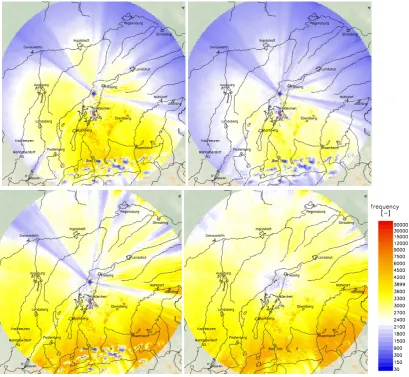
The result of the altitude correction is a homogeneous dis-tribution of frequencies of occurrence including rain patterns with areas of higher and lower frequencies of occurrence. The mean frequencies of occurrence are not dependent on the position of the radar any more as range dependence is not considered natural, but taken as bias. Figure 11 (bottom-left) shows the result for Fig. 3 (middle) after the altitude cor-rection for level 3, which obviously reveals significant im-provement. But still, clutter influence remains; the second correction should solve this problem. An application and a validation of the altitude correction and the following clutter correction and adjustment can be found in Sect. 6.
5.2 Correction of clutter effects and disturbances
Fig. 11. Result of the statistical correction of the frequencies of occurrence of reflectivities (level 3) of the Munich weather radar from 2000–2006 (PX data) – top left: uncorrected, top right: adjusted, bottom left: adjusted and altitude correction, bottom right: adjusted, altitude correction and correction of clutter and disturbances.
reflectivity of rain is, the more the influence of clutter domi-nates. The number of pixels that are corrupted by clutter de-creases significantly when the reflectivity inde-creases. There-fore, the correction also has to depend on reflectivity.
First, corrupted and uncorrupted pixels are separated for each reflectivity level class. As the frequencies of occurrence of radar reflectivities of level 5 and 6 are too low to be statis-tically analysed, the selection of corrupted pixels of level 4 is adopted for these heavy rain levels. This separation described in Sect. 3 is similar to the one used in Sect. 4 for level 1 using an empirical distribution technique.
One main aim of the correction is to preserve the reliable natural precipitation patterns. Two ways to deal with clutter affected pixels seems reasonable and were both used here. The first one is an interpolation algorithm for clutter affected pixels using values of the neighbours. The second one is a kind of adjustment, where frequencies of occurrence of radar
reflectivities are shifted to a higher level. This kind of correc-tion is mainly used for spokes.
to the median of the frequencies of all uncorrupted pixels of the adjacent 20–30 azimuth angles. The ratio of the two medians is calculated, which then serves as a correction fac-tor. These factors vary between 1.1 and 1.5. The two spokes east of the radar are caused by departing or landing planes and must, therefore, be completely interpolated. The im-provements according to this correction module are shown in Fig. 11 (bottom-right).
5.3 Adjustment
The adjustment is necessary to correct the uncertainties re-lated to the calculation of rain amounts from radar measure-ments. Additionally, for the presented correction algorithm the overrating caused by the altitude correction has to be corrected. Therefore, a stable adjustment to the mean rain amounts of rain gauges was realised.
The adjustment is based on the DX product and represents the third module of the statistical correction scheme. Here, rain amounts are compared instead of frequencies of occur-rence. So the radar data has to be converted into rain rate by the three-part Z/R-relationship in Table 2. Then mean annual rain amounts from radar data were compared to rain amounts from rain gauges for the time span 2004–2006.
For the adjustment only the 33 rain gauges within a dis-tance of 30 to 60 km from the radar (group 1) are used. Radar pixels in this area are highly reliable as these pix-els are neither influenced by city nor mountain clutter, but are still close to the radar site. The rest of the rain gauges (group 2 and group 3) were used in Sect. 6 for evaluation. So the rain amounts of the 33 rain gauges were compared to the corresponding rain amounts derived from radar reflectivities (9-pixel-value) resulting in a common mean adjustment fac-tor. A locally varying factor would probably distort measured precipitation patterns radar climatology usually aims at.
The adjustment factor is calculated on an annual rain amount, whereas correction module 1 (altitude correction) and module 2 (correction of clutter and disturbances) are based on frequencies of occurrence. To apply the adjustment factor also for frequencies of occurrence of radar reflectivi-ties an assumption has to be made: an integral rain amount (e.g., annual rain amount) is considered to be the product of the rain amount calculated from radar reflectivity times the corresponding frequency. For example, if the adjustment fac-tor is two, the rain amounts calculated from radar reflectivi-ties by the three-part Z/R-relation must be halved. The same quantitative result may also be achieved by halving the abso-lute frequencies of occurrence for each radar reflectivity class instead. This does not change the relative frequency distribu-tion of radar reflectivity classes which have so far been nor-malised to the arbitrary value ofY0. Consequently, the
adjust-ment factor can be applied to frequencies in order to integrate the rain amount of the respective class, as long as the calcu-lation of rain rate is performed by a static Z-R-recalcu-lationship.
The frequency of occurrence of radar reflectivities is then simply divided by this factor. This factor was determined for the corrected radar data as well as for the uncorrected radar data. Regarding long-term measurements, a good mean con-sistency between measurements from radar and rain gauges becomes obvious. For the uncorrected data a factor of 0.94 was determined whereas for corrected data a factor of 1.26 resulted (cf. Fig. 11 top-right). Again, the latter factor in-cludes the arbitrary factor Y0and must not be valued as
infe-rior to the former factor.
Figure 11 shows the results of the full correction algorithm for the Munich weather radar of radar reflectivity level 3. The visual impression reveals now a relatively homogeneous dis-tribution of frequencies of occurrence of radar reflectivities over the whole image, but is still conserving meteorologi-cally or geographimeteorologi-cally induced minima and maxima of rain. The comparable frequencies of occurrence of radar reflectivi-ties within the whole radar image are indications for an effec-tive and successful correction. In order to prove the quality of the correction algorithm a comparison with rain amounts from rain gauges was performed and results summarised in the following section.
6 Evaluation of the method
6.1 Application of the method
All modules are stand-alone corrections. Of course, e.g., the altitude correction should not be applied without the adjust-ment as it tends to overrate the true frequencies of occurrence of radar reflectivities. All corrections are performed on fre-quencies of occurrence of radar reflectivities. Only after the corrections rain amounts can be calculated from the corrected frequencies of occurrence of reflectivities.
For the following diagrams, we ordered the corrections from gauge adjustment, altitude correction to correction of clutter and disturbances in order to demonstrate the improve-ment with each step of correction. One side effect of the al-titude correction is an overestimation of the total frequencies of occurrence of radar reflectivities. The presented order in this chapter has no side effects on the results itself.
The annual rain amounts derived from radar measurements (9-pixel-value) is opposed to the annual rain amounts of rain gauges (group 2) of 2004 to 2006. The 76 measurements were further subdivided into five groups according to their distance from the radar (every 20 km) representing the prob-able modification of radar rain amounts with distance from the radar.
Figures 12 and 13 show each step of correction of radar data in comparison to rain gauges.
Fig. 12. Scatterplot of radar and rain gauge pairs of values for the statistical correction of reflectivity level 3 of the Munich weather radar from 2004–2006 (DX data). Each row shows one step of the correction algorithm: (a) uncorrected, (b) adjusted, (c) adjusted and altitude corrected, d) adjusted, altitude correction and correction of clutter and disturbances. The radar and rain gauge pairs of values are subdivided into five classes according to their distance from the radar site. Each column represents one range class: 0–20 km, 20–40 km, 40–60 km, 60–80 km and 80–100 km.
Fig. 13. Same data as for Fig. 12 but Box-and-Whisker-Diagram. The percential difference between radar data and rain gauge for each range class is shown. The thick bar indicates the median of each range class. The boxes show the deviation of 50 % of all radar and rain gauge pairs of values of one class. The whiskers mark 1.5 times the corresponding interquartile range or, if not reached, the maximum deviation.
algorithm, starting with the uncorrected data (a), adjusted radar data (b), additional altitude correction (c) and full cor-rection (d). Figure 13 shows the same comparison in a Box-and-Whisker-Diagram with five boxes starting with the 0– 20 km-class. The boxes and whiskers mark the percential dif-ference of radar measurements in comparison with the cor-responding rain gauge measurements for each range class. The first diagram shows the uncorrected mean annual rain amounts in class 1 (inner 20 km). While two measurements
[image:13.595.56.542.438.540.2]Table 3. RMSE of mean annual rain amounts of radar and rain gauge data in Fig. 12.
uncor (*) cor-b (**) cor-ba (***) cor-bac (****)
RMSE (mm) 262.1 359.3 126.4 118.3
* uncorrected radar data; ** corrected radar data (bias/adjusted); *** corrected radar data (bias/adjusted, altitude); **** corrected radar data (bias/adjusted, altitude, clutter).
for level 1 to level 4), where the regression line of the al-titude correction does not really represent this behaviour. But nevertheless the results from class 1 have to be handled with care. Classes 2 and 3 represent the most reliable areas within the radar-coverage with an excellent consistency of mean annual rain amounts of radar data and data from rain gauges. The three-part Z-R-relationship used to calculate rain amounts from reflectivity measurements is based on long-term measurements. The best agreement of measurements from radar and from gauges can be expected for long-term measurements, even though systematically induced varia-tions may add up. It is well known from radar hydrology, that for shorter time-spans much higher mean differences between radar measurements and gauge measurements oc-cur. Classes 4 and 5 reveal a significant underestimation of rain amounts by radar measurements. According to Fig. 13, a mean underestimation of 20 % in class 4 can be found, whereas in class 5 the underestimation is twice as high as in class 4 (40 %). It can be attested, that the decrease of rain amounts by radar measurements with distance from the radar on average is a measuring effect of the radar, whereas the rain amounts based on rain gauges are independent from this dis-tance.
With the statistically derived mean factor adjustment the radar measurements were shifted to a lower rain amount level in row b) of Fig. 12. For all classes a significant underestima-tion of rain amounts derived by radar measurements results. The RMSE rises from 262.1 mm to 359.3 mm (cf. Table 3). The second diagram of Fig. 13 reveals mean underestima-tions between 20 % and 50 % by radar data. Without the sub-sequent correction modules this correction leads to an im-pairment of data quality. Using the adjustment factor of 0.94 for uncorrected data a slight improvement of the RMSE to 247.3 mm becomes obvious (not shown here).
After the altitude correction a significant improvement of the consistency of measurements from radar and rain gauges becomes apparent (cf. row c) in Fig. 12). Especially range classes 4 and 5, where the altitude correction shows the greatest impact on the rain amounts, are improved, both vi-sually and based on statistical values. The RMSE changes from 262.1 mm (uncorrected data) to 126.4 mm. The Box-and-Whisker-Diagram supports these results. The maximum deviations of the median of radar rain amounts from the me-dian of gauge rain amounts at each range class decrease from a span of −40 % to +2 % (uncorrected data) to a span of −15 % to +3 % (corrected data).
Row d of Fig. 12 shows the results after the full correc-tion including the correccorrec-tion of spokes and cluttered pix-els. The RMSE (118.3 mm) indicates the further improve-ment as the diagram itself visually does. The maximum de-viations of the median of radar rain amounts from the me-dian of rain amounts from rain gauges of each range class decrease to a span of −5 % to +5 %. A comparison of the diagrams in row d with the diagrams in row a shows a sig-nificant improvement for all range classes. The greater the distance from the radar site the higher the deviations of rain amounts between measurements from radar and rain gauges. But even at a distance of 80 to 100 km (class 5) the max-imum range of deviation of mean rain amounts is −28 % to +33 % for all 76 pairs of values. This appears to be a small range, taking into account that measurements from rain gauges are affected by measuring problems with wind and snow or representativeness errors such as different sampling volumes and measurement heights. They may, therefore, dif-fer from radar measurements. In addition the geography of the Munich radar coverage is very difficult concerning mea-surements of rain amounts.
6.2 Validation of the method
For the validation of the presented correction algorithm the same comparisons of mean annual rain amounts from radar measurements and rain gauges are used, but for the time span 2007 to 2009 and for all available 91 pairs of val-ues (group 3). This also includes pairs of valval-ues in areas where the rain amounts do not seem reliable or where radar measurements are obviously disturbed by clutter effects and have, therefore, been interpolated by measurements in the closer vicinity. The very southern part within the range of the Alps usually shows higher rain amounts especially at higher altitudes. The interpolation does not take these effects into account, so a massive underestimation of rain amounts by radar measurements in comparison to rain gauge data in this area is likely. A second problematic area is the inner part of the radar coverage. Major parts of range class 1 cover the city of Munich with clutter problems. The results are presented in Figs. 14 and 15.
The three diagrams of Fig. 14 are comparable to those in Fig. 13, but for all pairs of values. Comparisons of rain amounts from uncorrected radar data of the years 2007 to 2009 in the first diagram are opposed to corrected radar data (2007–2009) in the second diagram. The third diagram shows the identical comparison as diagram 2, but for the years 2004 to 2006.
Fig. 14. Box-and-Whisker-Diagram of all radar and rain gauge pairs of values for the statistical correction of reflectivity level 3 of the Munich weather radar – left: uncorrected (2007–2009, validation period), middle: full correction (2007–2009, validation period), right: full correction (2004–2006, calibration period) (DX data).
Fig. 15. Mean annual rain amounts derived from the DX radar product of the Munich weather radar 2007–2009 – left: uncorrected, right: corrected.
of rain amounts with distance from the radar becomes clearly apparent in classes 4 and 5.
Diagram 2 (middle) shows the result of the full correc-tion algorithm. A significant improvement becomes obvious, both visually and based on the RMSE, which decreases from 322.2 mm to 174.1 mm (cf. Table 4). As expected, some pairs of values show only poor consistency. Most of them are lo-cated in the alpine area. The interpolated radar data is not able to reproduce the high rain amounts measured by rain gauges. The boxes and whiskers of diagram 2 show compa-rable ranges as diagram 4 of Fig. 12 does.
In diagram 3 (right) the same 91 pairs of values are com-pared for the calibration period to get evidence which part of the impairment of the results are based on the additional pairs of values and which part is based on the new time span. Diagram 3 shows a higher impairment than diagram 2 does. The RMSE of the validation period (RMSE=174.1 mm) is smaller than the RMSE of the calibration period (RMSE= 234.6 mm). So the impairment of the RMSE of 91 pairs of values of the validation period compared to the RMSE of the
Table 4. RMSE of mean annual rain amounts of radar and rain gauge data in Fig. 14.
uncor (*) cor-bac (****) cor-bac (****) (2007–2009) (2007–2009) (2004–2006)
RMSE (mm) 322.2 174.1 234.6
* uncorrected radar data; **** corrected radar data (bias/adjusted, altitude, clutter)
76 pairs of values of the calibration period (see Table 3) is mainly induced by the additional pairs of values.
[image:15.595.315.541.496.538.2]Figure 15 serves as a final visual validation of the results of the full correction algorithm. It shows the mean annual rain amounts derived from DX radar products before (left) and after the statistical corrections (right). The right panel of Fig. 15 shows the result after the full correction algo-rithm, for which the correction is based on frequencies of occurrence of DX data and calculated to rain amounts after-wards. The image shows a map of mean annual rain amounts which is very similar to maps of annually rain amounts based on point measurements (not shown here). The highest rain amounts are measured in the Alps and on the fringe of the Alps decreasing to the north. The radar image still reveals some remnants caused by clutter (e.g., City of Munich) or spokes.
7 Summary
We presented a statistical analysis of disturbances and the in-fluence of measuring effects on long-term precipitation radar measurements. Based on these findings a stable, statistical correction algorithm was derived. A significant improvement due to these corrections is shown using a comparison of radar precipitation data with rain gauges on an annual basis.
The statistical analysis of radar data on a seven-year tem-poral scale showed small systematic differences within a radar coverage, leading to recognisable accumulated errors in longer time series. For instance, the impact of beam-widening and increasing beam-height above ground with in-creasing range on the rain amounts can be seen on a long time range. The mean frequencies of occurrence of radar reflec-tivities as a function of height amount to−12.9 % per 1 km for reflectivity level 1 and−20.3 % per 1 km for level 2 to level 5, but are seasonally variable. A strong dependence on air-temperature becomes apparent. The transition from snow to rain combined with the bright band influence seems to be the main cause for this behaviour. According to these results, it is indispensable to include the correction of the VPR if radar data are to be applied over a longer time range, for ex-ample as input for a hydrological model in the water balance mode. The bright band should be negligible for heavy pre-cipitation in convective cells as convective cells usually have a large vertical homogeneity of rain. There are some indica-tions for that effect within this analysis, but the frequency of occurrence of such high reflectivity levels is too low to be statistically robust.
The full presented correction algorithm is designed for cli-matological or statistical analysis with a temporal resolution larger than one year. It is used for frequencies of occurrence which can be transferred to rain amounts afterwards. It is noted that there are no corrections on individual radar images of the original radar products (e.g., PX product or DX prod-uct). In this way, climatological analyses of secondary radar products such as of DWD’s cell-tracking-product CON-RAD may be corrected by this statistical correction. This
possibility is particularly valuable, for example, for estab-lishing reliable hazard maps. The main impact of the pro-posed correction algorithm is due to the altitude correction (module 1) which strongly depends on mean air tempera-ture. Only for heavy precipitation the altitude correction may also be applied at shorter temporal resolutions than one year. The parts of the correction algorithm concerning clutter and spokes (module 2) and the adjustment (module 3) are also suitable for smaller time scales or even for single radar image corrections. Even though, only a mean correction is realised which does not consider the current meteorological condi-tions. The extent of the statistical correction depends on the previous correction procedures. The better the single radar images are corrected in advance, the fewer statistical tions are necessary afterwards. But relying only on correc-tions of single-radar images usually results in recognisable errors in radar climatology. On a large time scale remain-ing small differences from any of the possible corrections on single-radar images may accumulate to larger errors.
The application of the correction algorithms shows a sig-nificant improvement of radar data quality. These results are based on a comparison of annual rain amounts of rain gauges and corresponding radar measurements for the appli-cation (2004–2006) and validation (2007–2009) periods. The Root-Mean-Square-Error (RMSE) between both datasets de-creases from 262 mm to 118 mm for the application period excluding those pairs of values where the rain gauges are sit-uated in areas of obviously corrupted radar data. The results for the validation period are based on all pairs of values and show a decrease of the RMSE from 322 mm to 174 mm. Edited by: R. Uijlenhoet
References
Bartels, H., Weigl, E., Reich, T., Lang, P., Wagner, A., Kohler, O., and Gerlach, N.: Projekt RADOLAN – Routineverfahren zur Online-Aneichung der Radarniederschlagsdaten mit Hilfe von automatischen Bodenniederschlagsstationen (Ombrometer), Deutscher Wetterdienst, Hydrometeorologie, 2004.
Fabry, F. and Zawadzki, I.: Long-term radar observations of the melting layer of precipitation and their interpretation, J. Atmos. Sci., 52, 838–851, 1995.
Franco, M., Sanchez-Diezma, R., and Sempere-Torres, D.: Im-provements in weather radar rain rate estimates using a method for identifying the vertical profile of reflectivity from volume radar scans, Meteorol. Z., 15, 521–536, 2006.
Haase, G., Gjertsen, U., and Bech, J.: Weather radar data quality in Northern Europe: beam propagation issues, AMS Conference on Radar Meteorology, Albuquerque, Canada, available at: ams. confex.com/ams/pdfpapers/96070.pdf (last access: 4 November 2012), 2005.
Hand, W. H.: An object-oriented technique for nowcasting heavy showers and thunderstorms, Meteorol. Appl., 3, 31–41, 1996. Holleman, I.: Bias adjustment and long-term verification of
2007.
Joss, J. and Lee, R.: The application of radar-gauge comparisons to operational precipitation profile corrections, J. Appl. Meteorol., 34, 2612–2630, 1995.
Kitchen, M., Brown R., and Davies, A. G.: Real-time correction of weather radar data for the effects of bright band, range and oro-graphic growth in widespread precipitation, Q. J. Roy. Meteorol. Soc., 120, 1231–1254, 1994.
Koistinen, J.: Operational correction of radar rainfall errors due to vertical reflectivity profile, Proc. 25th Conf. on Radar Met., AMS, 91–94, 1991.
Koistinen, J., Kuitunen, T., Pulkkinen, S., Hohti, H., and Kotro, J.: Derivation of extreme event mesoscale area-intensity re-turn periods of rainfall based on a large sample of radar data, ERAD, Helsinki, Finland, available at: http://www.ymparisto.fi/ download.asp?contentid=85495 (last access: 4 November 2012), 2008.
Krajewski, W. F., Vignal, B., Seo, B.-C., and Villarini, G.: Statistical model of the range dependent error in radar-rainfall estimates due to the vertical profile of reflectivity, J. Hydrol., 402, 306–316, 2010.
Overeem, A., Holleman, I., and Buishand, T. A.: Derivation of a 10-year radar-based climatology of rainfall, J. Appl. Meteor., 48, 1448–1463, 2009.
Overeem, A., Buishand, T. A., Holleman, I., and Uijlenhoet, R.: Extreme-value modeling of areal rainfall from weather radar, Water Resour. Res., 46, W09514, doi:10.1029/2009WR008517, 2010.
Pedersen, L., Jensen, N. and Madsen, E.: Extreme rainfall statistics based on rain gauges and radar measurements, WRaH Greno-ble, France, available at: http://radar.dhigroup.com/publications/ Extremerainfallstatisticsbasedonraingaugesandradar.pdf (last ac-cess: 4 November 2012), 2008.
Rudolph, J., Friedrich, K. and Germann, U.: Relationship between radar-estimated precipitation and synoptic weather patterns in the European Alps. J. Appl. Meteor. Climatol., 50, 944–957. 2011. S´anchez-Diezma, R., Zawadzki, I., and Sempere-Torres, D.:
Identification of the bright band through the analysis of volumetric radar data, J. Geophys. Res., 105, 2225–2236, doi:10.1029/1999JD900310, 2000.
Vignal, B., Andrieu, H., and Creutin, H.: Identification of vertical profiles of reflectivity from volume scan radar data, J. Appl. Me-teorol., 38, 1214–1228, 1999.