Assessing parameter importance of the Common Land Model based on qualitative and quantitative sensitivity analysis

Hydrol. Earth Syst. Sci., 17, 3279–3293, 2013 www.hydrol-earth-syst-sci.net/17/3279/2013/ doi:10.5194/hess-17-3279-2013

© Author(s) 2013. CC Attribution 3.0 License.

EGU Journal Logos (RGB)

Advances in

Geosciences

Open Access

Natural Hazards

and Earth System

Sciences

Annales

Geophysicae

Nonlinear Processes

in Geophysics

Atmospheric

Chemistry

and Physics

Atmospheric

Chemistry

and Physics

Atmospheric

Measurement

Techniques

Atmospheric

Measurement

Techniques

Biogeosciences

Open Access Open Access

Biogeosciences

Discussions

Climate

of the Past

Open Access Open Access

Climate

of the Past

Discussions

Earth System

Dynamics

Open Access Open Access

Earth System

Dynamics

Geoscientific

Instrumentation

Methods and

Data Systems

Open Access

_{Geoscientific}

Instrumentation

Methods and

Data Systems

Geoscientific

Model Development

Open Access Open Access

Geoscientific

Model Development

Hydrology and

Earth System

Sciences

Hydrology and

Earth System

Sciences

Ocean Science

Open Access Open Access

Ocean Science

Discussions

Solid Earth

Open Access Open Access

Solid Earth

The Cryosphere

Open Access Open Access

The Cryosphere

Discussions

Natural Hazards

and Earth System

Sciences

Open Access

Discussions

Assessing parameter importance of the Common Land Model

based on qualitative and quantitative sensitivity analysis

J. Li1, Q. Y. Duan1, W. Gong1, A. Ye1, Y. Dai1, C. Miao1, Z. Di1, C. Tong2, and Y. Sun2

1_{College of Global Change and Earth System Science (GCESS), Beijing Normal University, Beijing, 100875, China} 2_{Lawrence Livermore National Laboratory, Livermore, CA 94551, USA}

Correspondence to: Q. Y. Duan ([email protected]), J. D. Li ([email protected])

Received: 27 December 2012 – Published in Hydrol. Earth Syst. Sci. Discuss.: 21 February 2013 Revised: 17 June 2013 – Accepted: 7 July 2013 – Published: 21 August 2013

Abstract. Proper specification of model parameters is

criti-cal to the performance of land surface models (LSMs). Due to high dimensionality and parameter interaction, estimating parameters of an LSM is a challenging task. Sensitivity anal-ysis (SA) is a tool that can screen out the most influential parameters on model outputs. In this study, we conducted pa-rameter screening for six output fluxes for the Common Land Model: sensible heat, latent heat, upward longwave radiation, net radiation, soil temperature and soil moisture. A total of 40 adjustable parameters were considered. Five qualitative SA methods, including local, sum-of-trees, multivariate adaptive regression splines, delta test and Morris methods, were com-pared. The proper sampling design and sufficient sample size necessary to effectively screen out the sensitive parameters were examined. We found that there are 2–8 sensitive param-eters, depending on the output type, and about 400 samples are adequate to reliably identify the most sensitive parame-ters. We also employed a revised Sobol’ sensitivity method to quantify the importance of all parameters. The total ef-fects of the parameters were used to assess the contribution of each parameter to the total variances of the model outputs. The results confirmed that global SA methods can generally identify the most sensitive parameters effectively, while lo-cal SA methods result in type I errors (i.e., sensitive param-eters labeled as insensitive) or type II errors (i.e., insensitive parameters labeled as sensitive). Finally, we evaluated and confirmed the screening results for their consistency with the physical interpretation of the model parameters.

1 Introduction

A land surface model (LSM) is an integral component of any numerical weather prediction (NWP) and climate models. The ability of an LSM to represent the land surface processes accurately and reliably depends on several factors (Duan et al., 2006). The first factor is the authenticity of the model structure (e.g., the equations or parameterization schemes of the model). The second is the quality of external forcing data and the initial and boundary conditions. The third is the ap-propriateness of the model parameter specification. How to estimate model parameters has received increasing attention from the hydrology and land surface modeling community over recent years (Franks and Beven, 1997; Gupta et al., 1999; Duan et al., 2001, 2003; Jackson et al., 2003; Liu et al., 2005; Hou et al., 2012).

algorithm (GA) (Goldberg, 1989) and shuffled complex evo-lution method (Duan et al., 1993)) impractical.

For the reasons above, we need to reduce the dimensional-ity by identifying which parameters have the most influence on model performance. Sensitivity analysis (SA) is a family of methods that are designed to identify the most sensitive (namely, influential) parameters from the insensitive ones (Saltelli et al., 2004). A good SA method is able to screen out the most sensitive parameters in a relatively low number of model runs (Tong and Graziani, 2008).

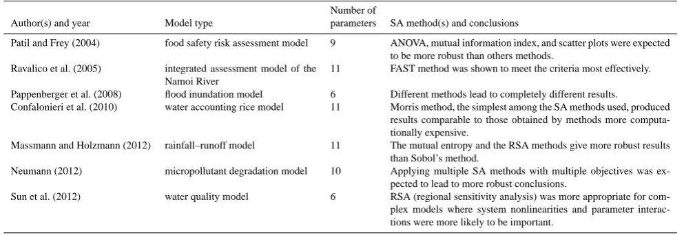
There are two types of SA methods: qualitative and quan-titative. Qualitative methods provide a heuristic score to intu-itively represent the relative sensitivity of parameters, while quantitative methods tell how sensitive the parameter is by computing the impact of the parameter on the total variance of model output. Qualitative methods usually need fewer model runs while quantitative methods require a large num-ber of model runs. Therefore, for a specific problem, choos-ing which kind of SA methods is very important. In recent decades, there are several comparisons of different SA meth-ods, of which seven examples are shown in Table 1. We can see that researchers have drawn different conclusions: some have suggested the quantitative SA methods are more re-liable, some maintain that the qualitative SA methods can achieve consistent results with the quantitative methods; and others have supposed that applying multiple SA methods would lead to more robust conclusions. This lack of con-sensus implies that more work is needed to answer how to choose the most appropriate SA method.

SA methods have been applied to practical problems in many fields (Campolongo and Saltelli, 1997; De Pauw et al., 2008; Yamwong and Achalakul, 2011). For hydrological and land surface models, Collins and Avissar (1994) employed the Fourier amplitude sensitivity test (FAST) to evaluate the parameter importance to the sensible heat and latent heat in the LAID (land–atmosphere interactive dynamic) land surface scheme. Bastidas et al. (1999) proposed the multi-objective generalized sensitivity analysis (MOGSA) method and screened out 18 sensitive parameters from a total of 25 parameters in the BATS (biosphere–atmosphere transfer scheme) model. It was demonstrated that the degradation in the quality of the calibrated model performance is negligi-ble if the insensitive parameters were not calibrated. Tang et al. (2007) applied local and global SA methods on the lumped Sacramento soil moisture accounting model (SAC-SMA). Their aim was to identify sensitivity tools that would advance the understanding of lumped hydrologic models. The relative efficiency and effectiveness of several SA meth-ods have been analyzed and compared. Hou et al. (2012) introduced an uncertainty quantification framework to ana-lyze the sensitivity of 10 hydrologic parameters in CLM4SP (Community Land Model Version 4 with satellite phenology) with a generalized linear model (GLM) method. They found that the simulation of sensible heat and latent heat is sensi-tive to subsurface runoff generation parameters. In the

afore-mentioned work, many SA methods have shown their effec-tiveness in screening out important parameters. However, for large complex dynamic system models, which are expensive to run, we need to be able to screen out important parameters with as few model runs as possible. Therefore, the goal of this study is to investigate the effectiveness and efficiency of different qualitative SA methods for parameter screening.

Several SA methods were used to evaluate the importance of 40 adjustable parameters in the Common Land Model (CoLM). The work has two objectives: (1) to test and com-pare different qualitative SA methods for separating sensi-tive parameters from insensisensi-tive ones; and (2) to validate the screening results using a quantitative SA method. Towards these objectives, this study first screened out the sensitive parameters qualitatively with a small amount of samples, and then quantified the sensitivity of all parameters using a quantitative SA method.

The paper is organized as follows. Section 2 presents a brief introduction of the qualitative SA methods for param-eter screening and the quantitative SA method for comput-ing the parameter importance. Section 3 introduces the model used, CoLM, and its adjustable parameters. The study area, the forcing and validation data, and the design of the sensi-tivity study are also described. Section 4 presents the results and discusses the performance of qualitative and quantitative SA methods. The physical interpretations of the screening re-sults are also examined. Section 5 provides the conclusions.

2 Methods

This study employed five qualitative SA methods to do pa-rameter screening: local method (Tur´anyi, 1990; Capaldo and Pandis, 1997), sum-of-trees (SOT) (Breiman, 2001; Chip-man et al., 2010), multivariate adaptive regression splines (MARS) (Friedman, 1991), delta test (DT) (Pi and Peterson, 1994) and Morris method (Morris, 1991). Moreover, to val-idate the parameter screening results obtained by qualitative methods, the revised Sobol’ method (Sobol’, 1993, 2001), was applied to compute the total effects of parameters. Be-low, we provide a brief description of these methods. For detailed descriptions, please refer to related literature.

2.1 Local method

Local method is a derivative-based sensitivity method. The sensitivity of variable Xi∈ [aibi] is computed as the

nor-malized local sensitivity scaled by the variable range: si =

1

(bi−ai) ∂Y

∂Xi|Xi=αi, wheresiis the local sensitivity measure,Y is the model output,αiis a value ofXi at which the

sensitiv-ity is evaluated, andaiandbiare the lower and upper bounds

ofXi. The variable with a highsi value is considered to have

a high impact on the model output. Obviously the value ofsi

Table 1. Comparison of different SA methods.

Number of

Author(s) and year Model type parameters SA method(s) and conclusions

Patil and Frey (2004) food safety risk assessment model 9 ANOVA, mutual information index, and scatter plots were expected to be more robust than others methods.

Ravalico et al. (2005) integrated assessment model of the Namoi River

11 FAST method was shown to meet the criteria most effectively.

Pappenberger et al. (2008) flood inundation model 6 Different methods lead to completely different results.

Confalonieri et al. (2010) water accounting rice model 11 Morris method, the simplest among the SA methods used, produced results comparable to those obtained by methods more computa-tionally expensive.

Massmann and Holzmann (2012) rainfall–runoff model 11 The mutual entropy and the RSA methods give more robust results than Sobol’s method.

Neumann (2012) micropollutant degradation model 10 Applying multiple SA methods with multiple objectives was ex-pected to lead to more robust conclusions.

Sun et al. (2012) water quality model 6 RSA (regional sensitivity analysis) was more appropriate for com-plex models where system nonlinearities and parameter interac-tions were more likely to be important.

2.2 Sum-of-trees (SOT) method

The SOT method is a tree-based method. A single regression tree model is a step function, which is obtained by recur-sively partitioning the data space and fitting a simple predic-tion model (generally, the average value) within each parti-tion (Breiman et al., 1984). In the process of recursively par-titioning, the variables are split to cause maximum decrease in impurity function (residual sum of squares) until the impu-rity function falls below a threshold. The SOT model uses a certain number of bootstrapped samples to build independent regression trees and then averages them (Breiman, 2001). The total number of splits for each variable in the model stands for the importance of this variable, i.e., the variable with the most splits in the model is considered to be the most important one.

2.3 Multivariate adaptive regression splines (MARS) method

The MARS method (Friedman, 1991; Shahsavani et al., 2010) is an extension of the regression tree method. After recursively partitioning the data space, it builds localized re-gression models (first-order linear or second-order nonlinear) instead of step functions. Therefore, this method can produce continuous models with continuous derivatives and has bet-ter fitting ability. This method includes a forward procedure and a backward procedure. The forward procedure builds an over-fitted model by considering all variables, while the backward procedure prunes the over-fitted model by remov-ing one variable at a time. For each modelM, a generalized cross-validation (GCV) score can be computed:

GCV(M)= 1 N

N P

i=1

Yi− ˆYi

2

h

1−C(M) N

i2 (1)

whereN is the number of observations,Yi is theith

obser-vation,Yˆiis the estimated value ofYi,C (M), which is equal

to 1+c (M) d, is the number of effective parameters, where d is the effective degrees of freedom, andc (M)is a penalty for adding a basic function.

To screen out the important variables, the increase in GCV values between the pruned model and the over-fitted model is considered as the importance measure of the removed vari-able (Steinberg et al., 1999). The larger the GCV increase, the more important is the removed variable.

The MARS method is actually a surrogate-model method. Shahsavani et al. (2010) showed that MARS provides accept-able estimates of total sensitivity indices at a much lower cost than using only runs of the original model.

2.4 Delta test (DT) method

DT method is a variable selection method based on the near-est neighbor approach. LetY =F (X)=F (X1, . . . , Xm)+ ε, where the noise ε=(ε1, . . . , εm), εi(i=1, . . . , m) is

independent identically distributed random variable with zero mean. The DT criterion of a variable subset S⊆ {X1, . . ., Xm},δ (S), can be computed as

δ (S)= 1 2N

N X

i=1

(YNS(i)−Yi)

2 ₍₂₎

whereNS(i)=arg mink6=i

Xi−Xk

2

Srepresents the nearest

neighbors of the input pointXifor the subsetS,YNS(i)is the function value corresponding to NS(i), Yi is the function

Table 2. Adjustable parameters and their ranges.

Index Parameter Physical meaning Category Unit Range

P1 dewmx maximum ponding of leaf area canopy – [0.05, 0.15]

P2 hksati saturated hydraulic conductivity soil mm s−1 [0.001, 1]

P3 porsl Porosity, fraction of soil mass that is voids soil – [0.25, 0.75]

P4 phi0 minimum soil suction soil mm [50, 500]

P5 wtfact fraction of shallow groundwater area soil – [0.15, 0.45]

P6 bsw Clapp and Hornberger “b” parameter soil – [2.5, 7.5]

P7 wimp a factor for controlling whether water is impermeable soil – [0.01, 0.1]

P8 zlnd roughness length for soil surface soil m [0.005, 0.015]

P9 pondmx maximum ponding depth for soil surface soil mm [5, 15]

P10 csoilc drag coefficient for soil under canopy soil – [0.002, 0.006]

P11 zsno roughness length for snow snow – [0.0012, 0.0036]

P12 capr tuning factor of soil surface temperature soil – [0.17, 0.51]

P13 cnfac Crank Nicholson factor canopy – [0.25, 0.5]

P14 slti slope of low temperature inhibition function canopy – [0.1, 0.3] P15 hlti 1/2 point of low temperature inhibition function canopy – [278, 288] P16 shti slope of high temperature inhibition function canopy – [0.15, 0.45] P17 sqrtdi the inverse of square root of leaf dimension canopy – [2.5, 7.5] P18 effcon quantum efficiency of vegetation photosynthesis canopy molCO2/molquanta [0.035, 0.35]

P19 vmax25 maximum carboxylation rate at 25◦ canopy – [10e-06, 200e-06]

P20 hhti 1/2 point of high temperature inhibition function canopy – – [305, 315] P21 trda temperature coefficient of conductance-photosynthesis model canopy – [0.65,1.95] P22 trdm temperature coefficient of conductance-photosynthesis model canopy – [300, 350] P23 trop temperature coefficient of conductance-photosynthesis model canopy – [250, 300]

P24 gradm slope of conductance-photosynthesis model canopy – [4, 9]

P25 binter intercept of conductance-photosynthesis model canopy – [0.125, 0.375]

P26 extkn coefficient of leaf nitrogen allocation canopy – [0.5, 0.75]

P27 chil leaf angle distribution factor canopy – [-0.3, 0.1]

P28 ref(1,1) shortwave reflectance of living leaf canopy – [0.07, 0.105]

P29 ref(1,2) shortwave reflectance of dead leaf canopy – [0.16, 0.36]

P30 ref(2,1) longwave reflectance of living leaf canopy – [0.35, 0.58]

P31 ref(2,2) longwave reflectance of dead leaf canopy – [0.39, 0.58]

P32 tran(1,1) shortwave transmittance of living leaf canopy – [0.04, 0.08]

P33 tran(1,2) shortwave transmittance of dead leaf canopy – [0.1, 0.3]

P34 tran(2,1) longwave transmittance of living leaf canopy – [0.1, 0.3]

P35 tran(2,2) longwave transmittance of dead leaf canopy – [0.3, 0.5]

P36 z0m aerodynamic roughness length canopy m [0.05, 0.3]

P37 ssi irreducible water saturation of snow snow – [0.03, 0.04]

P38 smpmax wilting point potential canopy mm [−2.e5,−1.e5]

P39 smpmin restriction for min of soil potential soil mm [−1.e8,−9.e7]

P40 trsmx0 maximum transpiration for vegetation canopy mm s−1 [1.e-4, 100. e-4]

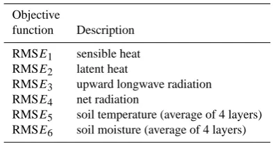
Table 3. The objective functions.

Objective

function Description

RMSE₁ sensible heat RMSE2 latent heat

RMSE₃ upward longwave radiation RMSE4 net radiation

RMSE5 soil temperature (average of 4 layers)

RMSE6 soil moisture (average of 4 layers)

criterion corresponds to the most important subset of vari-ables, i.e., the most sensitive parameters.

For high dimensional problems, it is impractical to com-pute all possible combinations of variable subsets (e.g., for 40 variables, the total configuration of subsets is 240−1). Therefore, to speed up the search for the variable subset with a minimumδ (S), search algorithms such as GA are often used (Guillen et al., 2008). Thus, the reliability of DT results depends on the effectiveness of the search algorithm applied.

2.5 Morris method

Fig. 1. The location of study area.

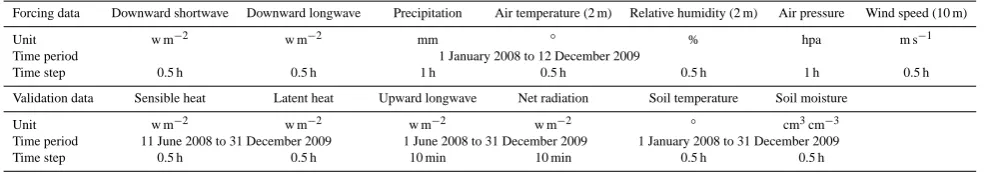
Table 4. The forcing data and validation data taken from A’rou observation station.

Forcing data Downward shortwave Downward longwave Precipitation Air temperature (2 m) Relative humidity (2 m) Air pressure Wind speed (10 m)

Unit w m−2 _{w m}−2 _mm ◦ _{% hpa m s}−1

Time period 1 January 2008 to 12 December 2009

Time step 0.5 h 0.5 h 1 h 0.5 h 0.5 h 1 h 0.5 h

Validation data Sensible heat Latent heat Upward longwave Net radiation Soil temperature Soil moisture

Unit w m−2 _{w m}−2 _{w m}−2 _{w m}−2 ◦ _cm3_cm−3

Time period 11 June 2008 to 31 December 2009 1 June 2008 to 31 December 2009 1 January 2008 to 31 December 2009

Time step 0.5 h 0.5 h 10 min 10 min 0.5 h 0.5 h

Note: the soil temperature and moisture data contain the data of 10, 20, 40, 80 and 120 cm, respectively.

withk independent inputs Xi (i=1, . . . , k), whose ranges

are normalized to [0, 1]. The experimentation region is a discretek-dimensionalp level grid. For a given value of pointX0=(x1, x2, . . . , xk), the elementary effect of variable Xj is defined as

dj=

f x1, . . ., xj+1, . . ., xk

−f (x1, . . ., xj, . . ., x_k)

1 , (3)

where1is a value in 1/p−1, . . ., p−2/p−1. The sam-pling strategy generates a random starting point for each tra-jectory and then completes it by perturbing one input vari-able by+1or−1at a time in a random order. At the end of process, a trajectory spanningk+1 points is evaluated to compute the elementary effects for allkinput variables. After repeating this procedurertimes to constructrtrajectories of k+1 points in the input space, the total cost of the experiment is thusr×(k+1). The mean of|d_j|,µj, and the standard

de-viation ofdj,σj, can be construed as the sensitivity indices

of input variableXj:

µj= r X

i=1

|dj(i)|/r and σj= v u u u u t r X

i=1

(dj(i)− r P

i=1 dj(i)

r )

2_{/r (4)}

Table 5. The depth of each layer.

layer 1 2 3 4 5 6 7 8 9 10

depth(cm) 0.71 2.79 6.23 11.89 21.22 36.61 61.98 103.80 172.76 286.46

whereµjassesses the overall influence ofXjon the output,

whileσj estimates the higher order effects (i.e., effects due

to interactions) ofXj.

Because of its characteristics of small computational de-mands, Morris method has been widely applied. Herman et al. (2013) demonstrated that it was able to correctly identify sensitive and insensitive parameters for a highly parameter-ized, spatially distributed watershed model with 300 times fewer model evaluations than the Sobol’ method.

2.6 Sobol’ method

Sobol’ method (Sobol’, 1993) is a quantitative SA method based on the variance decomposition the-ory, which decomposes the variance of the output as V=

n P

i=1

Vi+ P

1≤i<j≤n

Fig. 2. The sensitivity score of sensible heat given by SOT. The length of needles, which range from 0 to 100, represents the sensi-tivity score of each parameter.

Fig. 3. The sensitivity score of sensible heat given by MARS. The length of needles represents the sensitivity score.

the total number of variables, and Vi represents the part

of variance of output which can be explained by the ith variable only,Vij represents the part of variance of output

which can be explained by the interaction of the ith and jth variables, V1,2...,n represents the part of variance of

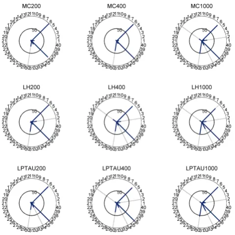
Table 6. The experiment designs to confirm the proper sampling methods and sample size for SA methods.

SA methods SOT MARS DT Morris

Sampling methods MC, LH, LPTAU MOAT Sample sizes 200, 400, 1000 205, 410, 1025

output which can be explained by the interaction of all the variables. The Sobol’ sensitivity index is defined as Si1,...,is =Vi1,...,is

V, where Vi1,...,is denotes the variance corresponding to (i1, . . . , is), and the integers is called the

order or the dimension of the index. All the values ofSi1,...,is are nonnegative, and their sum is

n X

i=1

Si+ X

1≤i<j≤n

Sij+. . .+S1,2...,n=1 (5)

whereSi=Vi

V is the main effect (first order effect) of the ith variable, andSij=VijV is the interaction effect

(sec-ond order effect) of theith andjth variables (Sobol’, 2001). The total effect of theith variable can be obtained by Eq. (6), whereV−i is the variance without considering thei-th

vari-able (Homma and Saltelli, 1996):

STi=1− V−i

V . (6)

The total effect reflects the variable’s contribution to the vari-ance of model output. The values of those indices for impor-tant variables are generally much higher than those for unim-portant ones.

Fig. 4. The sensitivity score of sensible heat given by DT. The length of needles represents the sensitivity score.

Fig. 5. The sensitivity score of sensible heat given by Morris method. The length of needles represents the sensitivity score.

To assess the importance of parameterP(i), we computed the relative values of the total effects of parameterP(i):

C (i)=STi/ n X

k=1

STk. (7)

The cumulative importance of a subset of parameters,A, can be computed as

˜

C (A)=X A

C (i). (8)

3 Experimental setup

3.1 CoLM and adjustable parameters

CoLM (Dai et al., 2003) is a widely used land surface model. It combines the advantages of three existing land sur-face models: Land Sursur-face Model (LSM) (Bonan, 1996), Biosphere-atmosphere transfer scheme (BATS) (Dickinson

et al., 1993) and Institute of Atmospheric Physics land-surface model (IAP94) (Dai and Zeng, 1997). In recent years, it has incorporated different physical processes such as glacier, lake, wetland and dynamic vegetation. It has also been successfully implemented in several global atmospheric models (Yuan and Liang, 2010).

CoLM considers the biophysical, biochemical, ecological and hydrological processes. The energy and water transmis-sion among soil, vegetation, snow and atmosphere is well described. The model contains one vegetation layer, 10 un-evenly distributed vertical soil layers, and up to five snow layers (depending on the snow depth). The parameteriza-tion scheme of soil thermal and hydraulic properties are de-rived from Farouki (1986), Clapp and Hornberger (1978) and Cosby et al. (1984). The parameterization scheme of snow is synthesized from Anderson (1976), Jordan (1991) and Dai et al. (1997).

In this study, forty of the time-invariant coefficients and exponents in CoLM, i.e., model parameters, are chosen as pa-rameters that can be adjusted according to local conditions. Their physical meanings and value ranges are shown in Ta-ble 2. These adjustaTa-ble parameters can be classified into three categories: canopy, soil and snow. The default parameters of canopy depend on the vegetation type in the 24-category (USGS) vegetation dataset. Soil parameters depend on the soil texture in the 17-category (FAO-STATSGO) soil dataset. Snow parameters depend on the snow depth. In this paper, the parameter ranges are the lower and upper bounds among all the possible types of canopy, soil and snow types (Ji and Dai, 2010). Note that the initial parameter ranges can have significant influence on the result of sensitivity analysis. For example, y=(a2+b)x where the range of input “x” and parameter “b” are both [0,1]. Obviously, parameter “a” is sensitive when the absolute value of “a” is very large, and insensitive when “a” is close to zero. The initial parameter ranges must be carefully selected and the analysis result may be valid only for these ranges. For convenience, these param-eters are index numbered from P1 to P40.

This study screens sensitive parameters for six land sur-face fluxes: sensible heat, latent heat, upward longwave radi-ation, net radiradi-ation, soil temperature and soil moisture. The objective function is the root-mean squared error normalized by the geometric mean (Parada et al., 2003):

RMSEi= s

N P

j=1

y_i,jsim−y_i,jobs

2

s N P

j=1

y_i,jobs2

(9)

Fig. 6. The qualitative sensitivity analysis results of different methods for sensible heat. The sensitivity scores are normalized to [0, 1]; 1 means most sensitive and 0 means least sensitive.

Fig. 7. The qualitative sensitivity analysis results of different methods for latent heat. The sensitivity scores are normalized to [0, 1]; 1 means most sensitive and 0 means least sensitive.

the performance of simulation, so a smaller RMSE means a better performance.

3.2 Study area and datasets

The Heihe River basin, the second largest inland river basin in the arid region of northwest China, is located be-tween 96◦420–102◦000E and 37◦410–42◦420N, and covers an area of approximately 130 000 km2. The Heihe River basin, whose altitude varies approximately from 0 to 5500 m, is covered by a variety of land use types, including desert, farm-land, forest, grassfarm-land, snow cap, etc. Therefore, it is an ideal region for the study of LSM. In this paper, A’rou observation station, which is located upstream of the Heihe River basin, is chosen for the study area. The results of SA methods inter-comparison will be helpful for following up research projects of the whole region. The geographic coordinate of A’rou is 100◦280E, 30◦080N (see Fig. 1); its altitude is 3032.8 m above sea level. It belongs to the typical continental climate. The underlying surface type is alpine steppe.

The forcing data and validation data is shown in Table 4. The forcing data of CoLM includes downward shortwave and longwave radiation, precipitation, air temperature, rel-ative humidity, air pressure and wind speed (Hu et al., 2008). The validation data contains observations of six fluxes. These six fluxes are all important physical quantities between land surface and atmosphere. Soil temperature and moisture data are available for depths of 10, 20, 40 and 80 cm. Because the soil column in CoLM is divided into 10 layers (the depths are

shown in Table 5), we used the linear interpolation method to achieve soil temperature and moisture calculations for the observed depths.

The data for year 2008 was used to spin up CoLM. Model simulations from 1 January 2009 to 31 December 2009 with a 3 h time step are used to evaluate model parameter sensitivity.

3.3 Design of sensitivity study

This study used a newly developed software package named Problem Solving environment for Uncertainty Anal-ysis and Design Exploration (PSUADE) (Tong, 2005) for all SA analyses. PSUADE implements various uncertainty quantification (UQ) tools such as design of experiments, sampling methods, qualitative and quantitative sensitiv-ity analysis, response surface, uncertainty assessment, and numerical optimization.

Fig. 8. The qualitative sensitivity analysis results of different methods for upward longwave radiation. The sensitivity scores are normalized to [0, 1]; 1 means most sensitive and 0 means least sensitive.

Fig. 9. The qualitative sensitivity analysis results of different methods for net radiation. The sensitivity scores are normalized to [0, 1]; 1 means most sensitive and 0 means least sensitive.

are also checked for their consistency with the parameters’ physical interpretations.

4 Results and discussion

4.1 Qualitative parameter screening

4.1.1 Sampling methods and sample sizes

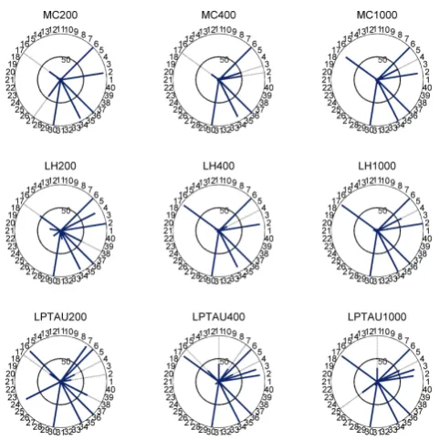
We tested and compared different sampling methods and sample sizes (see Table 6). For SOT, MARS and DT, three sampling methods were evaluated: Monte Carlo (MC) (Hast-ings, 1970), Latin Hypercube (LH) (McKay et al., 2000) and LPTAU (quasi random sequences) (Statnikow and Matusov, 2002). For each sampling method, different sample sizes, 200, 400 and 1000 (i.e., 5, 10 and 25 times of the number of parameters, respectively), were investigated. Morris method has its own sampling method. The sample size of Morris method is generally set as a multiple of n+1, where n is the number of parameters. Therefore this study tested three sample sizes: 205, 410 and 1025 for Morris method.

Take the results of SOT for example, which examines pa-rameters most sensitive to sensible heat flux. The SOT sen-sitivity scores of 40 parameters given by different sampling designs are shown in Fig. 2. The numbers along each cir-cle represent different parameters, with the length of the needles, which range from 0 to 100, indicating the relative sensitivities of different parameters.

From Fig. 2, we can see the most important parameters based on SOT method. With 1000 samples, all sampling methods identified the same sensitive parameters: P36, P6, P30, P2, P34 and P17. When the sample size is reduced to 400 for LH and LPTAU, the results are similar to those at 1000 samples, suggesting that a sample size of 400 is ade-quate for identifying the most sensitive parameters. With 400 samples, SOT based on MC sampling method can still screen out the same parameters, but the medium sensitive parame-ters, P2, P34 and P17, are not as clearly identified. With 200 samples, even though SOT using all the three sampling meth-ods can still find all sensitive parameters, the relative sensi-tivities of the medium sensitive parameters are too small to be seen clearly (e.g., P17). This suggests that 200 samples may not be enough for SOT method. Thus, LH and LPTAU are considered to be better sampling designs for SOT, and 400 samples are enough for these sampling designs.

Fig. 10. The qualitative sensitivity analysis results of different methods for soil temperature. The sensitivity scores are normalized to [0, 1]; 1 means most sensitive and 0 means least sensitive.

Fig. 11. The qualitative sensitivity analysis results of different methods for soil moisture. The sensitivity scores are normalized to [0, 1]; 1 means most sensitive and 0 means least sensitive.

400 for these three designs. For Morris method, the sample size is set to 410.

4.1.2 Intercomparison of qualitative SA methods

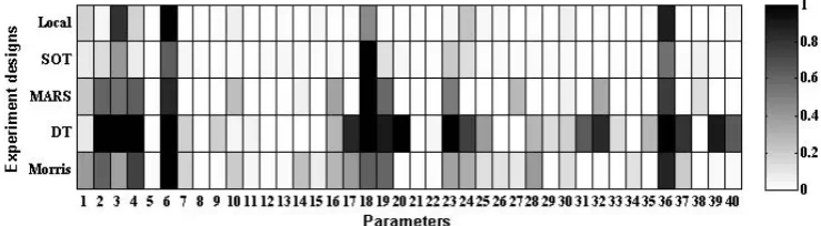
The parameter screening results by all qualitative SA meth-ods for all fluxes are summarized in Figs. 6–11. The sensitiv-ity scores of 40 parameters are normalized to [0, 1]. The most sensitive parameters get a score of 1, while the least sensitive ones get a 0 score. The vertical axis in these figures denotes different SA methods and the horizontal axis denotes the 40 parameters. The grey scale of each grid indicates the sensi-tivity level of each parameter by each SA method. In Fig. 6, for example, the dark grey color for P6 and P36 indicates that they are the most sensitive parameters for sensible heat flux. From these figures we have three interesting findings. First, for each land surface flux, the number of sensitive pa-rameters appears to be less than 10. For latent heat and sen-sible heat fluxes, there are more sensitive parameters as com-pared to other fluxes, which have only 2–3 sensitive parame-ters. Second, the results of SOT, MARS and Morris methods are consistent with each other except for the case of latent heat. For latent heat, the number of sensitive parameters is relatively larger than that of other fluxes (this is confirmed in the following quantitative SA). SOT, MARS and Morris methods got similar results for the most sensitive parameters, but there are some discrepancies in identifying the medium sensitive parameters for latent heat. Third, the results of Lo-cal method and DT appear very different from that of other

methods. Local method often takes sensitive parameters as insensitive ones (type I error, e.g., P3 for soil moisture) or the insensitive parameters as sensitive ones (type II error, e.g., P20 and P27 for sensible heat). The possible reason is that the local behavior near one specific parameter set is dif-ferent from the global behavior. The most sensitive param-eters given by DT are similar to other methods, but results for medium sensitive parameters are significantly different, especially when there are a large number of sensitive param-eters (e.g., in the cases of sensible heat and latent heat). We suspected that the GA used in DT failed to find the optimal parameter subset in those cases.

4.2 Validation of parameter screening results

Fig. 12. The relative importance of parameters obtained by RSMSobol’ total effect analysis.

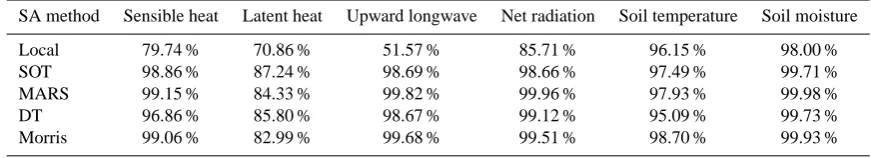
Table 7. The cumulative importance of the 10 most sensitive parameters screened by different qualitative SA methods.

SA method Sensible heat Latent heat Upward longwave Net radiation Soil temperature Soil moisture

Local 79.74 % 70.86 % 51.57 % 85.71 % 96.15 % 98.00 %

SOT 98.86 % 87.24 % 98.69 % 98.66 % 97.49 % 99.71 %

MARS 99.15 % 84.33 % 99.82 % 99.96 % 97.93 % 99.98 %

DT 96.86 % 85.80 % 98.67 % 99.12 % 95.09 % 99.73 %

Morris 99.06 % 82.99 % 99.68 % 99.51 % 98.70 % 99.93 %

less than 10 (i.e., 2–8). This confirms that the results of qual-itative SA methods are reasonable.

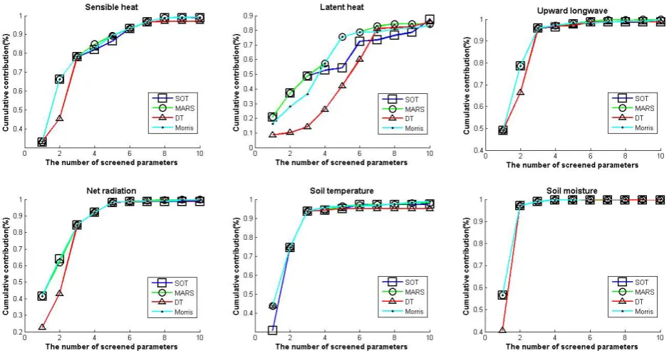
Table 7 shows the cumulative importance of the 10 most sensitive parameters selected by different qualitative SA methods, as computed according Eq. (8). The SA method is regarded as effective if the cumulative importance of the 10 most sensitive parameters is close to 100 %. Ob-viously, local method is ineffective in screening the im-portant parameters for sensible heat (79.74 %), latent heat (57.98 %), upward longwave radiation (51.57 %) and net ra-diation (85.71 %); while the other methods are effective be-cause the cumulative importance of the 10 most sensitive pa-rameters are close to 100 %. Furthermore, to confirm the ef-fectiveness of global SA methods, Fig. 13 shows the cumu-lative importance of the top 10 sensitive parameters screened by different SA methods. According to Fig. 13, the SOT, MARS and Morris methods performed well for all the land surface fluxes as their cumulative importance curves are always higher than others.

DT is prone to selecting more parameters than other meth-ods (committing type II error) and does not distinguish the medium sensitive from highly sensitive parameters. But the result of validation shows that the most sensitive parameters selected by DT are nearly the same to that given by the other global methods, even though the medium sensitive

parame-ters may differ from the ones identified by other SA methods. This suggests that a type II error possibly committed by DT is not as damaging as a type I error, as in the case of local method.

In summary, global SA methods, SOT, MARS, DT and Morris methods, are effective to reliably screen the most sen-sitive parameters with only 400 samples for a 40-parameters problem, even though DT may commit a type II error. Local gradient SA is helpful if we are interested in particular events or a special parameter set, but it might give misleading results when we are concerned about analyzing global behavior.

4.3 The consistency of the screening results and physical interpretations

In previous sections, we used five different qualitative SA methods to identify the most sensitive parameters for all flux types. The quantitative RSMSobol method confirms that the qualitative SA results are reasonable. Here we try to ex-plain the SA results based on physical interpretations of the screened parameters.

Fig. 13. The relationship between the number of screened parameters and cumulated relative importance for different sensitivity analysis methods.

hydraulic conductivity and water potential, and P3 (poros-ity) is a part of the denominator in the formulas that compute wetness. A small perturbation in these values would result in much change to soil moisture. Therefore these two param-eters are sensitive for soil moisture. It should be mentioned that P2 (saturated hydraulic conductivity) and P4 (minimum soil suction) will also affect the simulation of soil moisture (see Fig. 11), but they are not as sensitive as P6 and P3, which have an exponential relationship with soil moisture.

Besides soil moisture, P6 is also important for other land surface fluxes (see Fig. 12). This is because soil moisture is an important model output that is tied to sensible heat flux, la-tent heat flux and radiant fluxes (Henderson-Sellers, 1996). A parameter that exerts great influence on soil moisture should have an important impact on related fluxes. This finding is consistent with those of Lettenmaier et al. (1996).

P36 (aerodynamic roughness length) is another important parameter for sensible heat, latent heat, upward longwave radiation, net radiation and soil temperature (see Fig. 12). Through its influence on friction velocity, P36 affects the magnitude of aerodynamic resistance and near-surface drag force for the simulation of sensible heat, latent heat, and ra-diant fluxes, and therefore indirectly affects estimates of soil temperature (Dorman and Sellers, 1989). P17 (the inverse of square root of leaf dimension), P30 (longwave reflectance of living leaf) and P34 (longwave transmittance of living leaf) are sensitive to the simulations of surface temperature and air temperature. Accordingly, they are important for sensible heat and net radiation. The sensitivity of other parameters,

including P18 (quantum efficiency of vegetation photosyn-thesis) and P4 (minimum soil suction), to latent heat can be explained by their influence on evapotranspiration.

But not all the parameters in the screening results can be explained based on physical interpretations (e.g., P12 in screening result for latent heat). Possible reasons are (1) due to the limitation of the SA methods and the sample sizes as the insensitive parameters might be regarded as sensitive ones; (2) due to a lack of authenticity of the model struc-ture as the physical processes might not be described per-fectly; (3) due to local conditions or a lack of appropriate ob-servations for sensitivity evaluation (e.g., saturated hydraulic conductivity P2 is not sensitive because there is no runoff observations); (4) input uncertainty caused by observation error possibly having non-ignorable influence on the sensi-tivity analysis; (5) screening the sensitive parameters for a complex model may be a non-uniqueness issue.

5 Conclusions

results of the quantitative method are consistent with those of qualitative methods. Moreover, the screening results are generally consistent with the physical interpretations of the model parameters.

By using meteorological and land surface observation data in A’rou for the Heihe River basin in northwestern China, this study demonstrates the feasibility of employing differ-ent qualitative global SA methods to find the most important parameters in a complex model, which is similar to methods used by Massmann and Holzmann (2012). Though different methods are compared, we confirmed that global SA meth-ods are more suitable for complex models to screen out the most sensitive parameters from the insensitive ones. Because there exist some differences among the rank of screened pa-rameters given by different SA methods, we suggest that multiple SA methods be applied for a complex problem, which is also supported by Neumann (2012).

For a 40-parameter CoLM, we were able to screen out the most important parameters using only about 400 samples, which is similar to Confalonieri et al. (2010). The kind of parameter screening approach studied here should be appli-cable to other complicated models. However, caution must be exercised in interpreting these results. The parameters iden-tified in this study were obtained with data of limited length and at a single site with particular geographical conditions. Results from a different location or a different condition can be quite different from the ones shown in this study. The screened parameters are also tied to available land surface fluxes used in the study. Parameters such as saturated hy-draulic conductivity (P2) were not considered important pa-rameters because we did not examine parameter sensitivity to runoff generation. To truly understand the parameter sensitiv-ity for CoLM, we need to conduct a more comprehensive SA study by including more geographical locations, more ob-servation data types and longer datasets. In future research, parameter screening of CoLM will be extended to regional and even global scale by using more available data.

Even though we identified the most important parame-ters for CoLM, we did not perform model calibration to obtain the most appropriate estimates for these parameters. Model calibration for complex multi-flux, high-dimensional LSMs such as CoLM can be extremely complicated. To do model calibration in such cases, future studies must ex-plore more mathematical tools, including the surrogate mod-eling approach, to save computational resources and there-fore feasibly achieve a multi-objective optimization strategy for model calibration of multi-physics models.

Acknowledgements. The authors want to acknowledge the support provided by Natural Science Foundation of China (grant no. 41075075) and Chinese Ministry of Science and Technology 973 Research Program (grant no. 2010CB428402). Special thanks are due to the Environmental & Ecological Science Data Center for West China, National Natural Science Foundation of China (http://westdc.westgis.ac.cn) for providing the meteorological

forcing data, and to the group of Prof. Shaomin Liu at State Key Laboratory of Remote Sensing Science, School of Geography and Remote Sensing Science of Beijing Normal University, for providing the surface flux validation data.

Edited by: Z. Bargaoui

References

Anderson, E. A.: A point energy and mass balance model of a snow cover, NOAA Tech. Rep. NWS, 19, 1–150, 1976.

Bastidas, L. A., Gupta, H. V., Sorooshian, S., Shuttleworth, W. J., and Yang, Z. L.: Sensitivity analysis of a land surface scheme us-ing multicriteria methods, J. Geophys. Res., 104, 19481–19490, doi:10.1029/1999JD900155, 1999.

Bonan, G. B.: Land surface model (LSM version 1.0) for ecolog-ical, hydrologecolog-ical, and atmospheric studies: Technical descrip-tion and user’s guide, Technical note, Nadescrip-tional Center for At-mospheric Research, Boulder, CO (United States), Clim. Global Dynam. Div., 159 pp., 1996.

Breiman, L.: Random forests, Mach. Learn., 45, 5–32, doi:10.1023/A:1010933404324, 2001.

Breiman, L., Friedman, J., Stone, C. J., and Olshen, R. A.: Clas-sification and Regression Trees, Chapman and Hall/CRC, Bota Raton, Florida, USA, 1984.

Campolongo, F. and Saltelli, A.: Sensitivity analysis of an environ-mental model: an application of different analysis methods, Re-liab. Eng. Syst. Safe., 57, 49–69, 1997.

Campolongo, F., Cariboni, J., and Saltelli, A.: An effective screen-ing design for sensitivity analysis of large models, Environ. Mod-ell. Softw., 22, 1509–1518, 2007.

Capaldo, K. P. and Pandis, S. N.: Dimethylsulfide chemistry in the remote marine atmosphere: evaluation and sensitivity analysis of available mechanisms, J. Geophys. Res., 102, 23251–23267, 1997.

Chipman, H. A., George, E. I., and McCulloch, R. E.: BART: Bayesian additive regression trees, Ann. Appl. Stat., 4, 266–298, 2010.

Clapp, R. B. and Hornberger, G. M.: Empirical equations for some soil hydraulic properties, Water Resour. Res., 14, 601–604, doi:10.1029/WR014i004p00601, 1978.

Collins, D. C. and Avissar, R.: An evaluation with the Fourier am-plitude sensitivity test (FAST) of which land-surface parameters are of greatest importance in atmospheric modeling, J. Climate, 7, 681–703, 1994.

Confalonieri, R., Bellocchi, G., Bregaglio, S., Donatelli, M., and Acutis, M.: Comparison of sensitivity analysis techniques: a case study with the rice model WARM, Ecol. Modell., 221, 1897– 1906, 2010.

Cosby, B., Hornberger, G., Clapp, R., and Ginn, T.: A statistical exploration of the relationships of soil moisture characteristics to the physical properties of soils, Water Resour. Res., 20, 682–690, 1984.

Dai, Y. and Zeng Q.: A land surface model (IAP94) for climate studies part I: formulation and validation in off-line experiments, Adv. Atmos. Sci., 14, 433–460, doi:10.1007/s00376-997-0063-4, 1997.

R., and Niu, G.: The Common Land Model, Bull. Am. Meteorol. Soc., 84, 1013–1023, 2003.

De Pauw, D. J. W., Steppe, K., and De Baets, B.: Unravelling the output uncertainty of a tree water flow and storage model using several global sensitivity analysis methods, Biosyst. Eng., 101, 87–99, doi:10.1016/j.biosystemseng.2008.05.011, 2008. Deb, K., Pratap, A., Agarwal, S., and Meyarivan, T.: A fast and

eli-tist multiobjective genetic algorithm: NSGA-II, IEEE T. Evolut. Comput., 6, 182–197, 2002.

Dickinson, R., Henderson-Sellers, A., and Kennedy, P.: Biosphere– Atmosphere Transfer Scheme (BATS) version 1e as coupled to the NCAR community model, NCAR Tech. Note NCAR/TN-387 + STR, National Center for Atmospheric Research, Boulder, CO, USA, 72, 1993.

Dorman, J. and Sellers, P. J.: A global climatology of albedo, rough-ness length and stomatal resistance for atmospheric general cir-culation models as represented by the Simple Biosphere Model (SiB), J. Appl. Meteorol., 28, 833–855, 1989.

Duan, Q. Y., Gupta, V. K., and Sorooshian, S.: Shuffled com-plex evolution approach for effective and effcient global minimization, J. Optimiz. Theory App., 76, 501–521, doi:10.1007/BF00939380, 1993.

Duan, Q., Schaake, J., and Koren, V.: A priori estimation of land surface model parameters, land surface hydrology, meteorology, and climate: observations and modeling, Water Sci. Appl., 3, 77– 94, 2001.

Duan, Q., Gupta, H. V., Sorooshian, S., Rousseau, A. N., and Tur-cotte, R.: Calibration of Watershed Models, American Geophys-ical Union, Washington, USA, 345, 2003.

Duan, Q., Schaake, J., Andreassian, V., Franks, S., Goteti, G., Gupta, H. V., Gusev, Y. M., Habets, F., Hall, A., Hay, L., Hogue, T., Huang, M., Leavesley, G., Liang, X., Nasonova, O. N.,Noilhan, J., Oudin, L., Sorooshian, S., Wagener, T., and Wood, E. F.: Model Parameter Estimation Experiment (MOPEX): an overview of science strategy and major results from the second and third workshops, J. Hydrol., 320, 3–17, doi:10.1016/j.jhydrol.2005.07.031, 2006.

Eirola, E., Liiti’ainen, E., Lendasse, A., Corona, F., and Verleysen, M.: Using the delta test for variable selection, In: Proceedings of ESANN 2008/16th European Symposium on Artificial Neural Networks, Bruges (Belgium), 23–25 April 2008, 25–30, 2008. Farouki, O. T.: Thermal properties of soils, Ser. Rock Soil Mech.,

11, 1–136, 1986.

Franks, S. W. and Beven, K. J.: Bayesian estimation of uncertainty in land surface-atmosphere flux predictions, J. Geophys. Res., 102, 23991–23999, doi:10.1029/97JD02011, 1997.

Friedman, J. H.: Multivariate adaptive regression splines, Ann. Stat., 19, 1–141, 1991.

Goldberg, D.: Genetic Algorithms in Search, Optimization, and Machine Learning, Addison-Wesley Professional, Boston, MA, USA, 1989.

Guillen, A., Sovilj, D., Lendasse, A., and Mateo, F.: Minimizing the delta test for variable selection in regression problems, Int. J. High Perform. Sys. Arch., 1, 269–281, 2008.

Gupta, H., Bastidas, L., Sorooshian, S., Shuttleworth, W., and Yang, Z.: Parameter estimation of a land surface scheme using multicri-teria methods, J. Geophys. Res., 104, 491–503, 1999.

Hastings, W. K.: Monte Carlo sampling methods using Markov chains and their applications, Biometrika, 57, 97–109, 1970.

Henderson-Sellers, A.: Soil moisture: a critical focus for global change studies, Global Planet. Change, 13, 3–9, 1996.

Herman, J. D., Kollat, J. B., Reed, P. M., and Wagener, T.: Tech-nical note: Method of Morris effectively reduces the computa-tional demands of global sensitivity analysis for distributed wa-tershed models, Hydrol. Earth Syst. Sci. Discuss., 10, 4275– 4299, doi:10.5194/hessd-10-4275-2013, 2013.

Homma, T. and Saltelli, A.: Importance measures in global sensi-tivity analysis of nonlinear models, Reliab. Eng. Syst. Safe., 52, 1–17, 1996.

Hou, Z., Huang, M., Leung, L. R., Lin, G., and Ricciuto, D. M.: Sensitivity of surface flux simulations to hydrologic parame-ters based on an uncertainty quantification framework applied to the Community Land Model, J. Geophys. Res., 117, D15108, doi:10.1029/2012JD017521, 2012.

Hu, Z. Y., Ma, M. G., Jin, R., Wang, W. Z., Huang, G. H., Zhang, Z. H., and Tan, J. L.: WATER: dataset of automatic meteorological observations at the A’rou freeze/thaw observa-tion staobserva-tion, Cold and Arid Regions Environmental and En-gineering Research Institute, Chinese Academy of Sciences, doi:10.3972/water973.0279.db, 2008.

Jackson, C., Xia, Y., Sen, M. K., and Stoffa, P. L.: Optimal param-eter and uncertainty estimation of a land surface model: a case study using data from Cabauw, Netherlands, J. Geophys. Res., 108, 4583, doi:10.1029/2002JD002991, 2003.

Ji, D. Y. and Dai, Y. J.: The Common Land Model (CoLM) technical guide, Technical Report of Beijing Normal University, Beijing, China, 2010.

Jordan, R.: A one-dimensional temperature model for a snow cover: technical documentation for SNTHERM, 89, DTIC Document, US Army Cold Regions Research and Engineering Laboratory Special Rep., USA, 91–16, 1991.

Lettenmaier, D., Lohmann, D., Wood, E., and Liang, X.: PILPS-2c workshop report, Princeton Univ., Princeton, NJ, 1996. Liu, Y., Gupta, H. V., Sorooshian, S., Bastidas, L. A., and

Shut-tleworth, W. J.: Constraining land surface and atmospheric pa-rameters of a locally coupled model using observational data, J. Hydrometeorol., 6, 156–172, 2005.

Massmann, C. and Holzmann, H.: Analysis of the behavior of a rainfall–runoff model using three global sensitivity analysis methods evaluated at different temporal scales, J. Hydrol., 475, 97–110, 2012.

McKay, M., Beckman, R., and Conover, W.: A comparison of three methods for selecting values of input variables in the analysis of output from a computer code, Technometrics, 42, 55–61, 2000. Morris, M. D.: Factorial sampling plans for preliminary

computa-tional experiments, Technometrics, 33, 161–174, 1991. Neumann, M. B.: Comparison of sensitivity analysis methods for

pollutant degradation modelling: A case study from drinking wa-ter treatment, Sci. Total Environ., 433, 530–537, 2012.

Pappenberger, F., Beven, K. J., Ratto, M., and Matgen, P.: Multi-method global sensitivity analysis of flood inundation models, Adv. Water Resour., 31, 1–14, 2008.

Parada, L. M., Fram, J. P., and Liang, X.: Multi-resolution calibra-tion methodology for hydrologic models: applicacalibra-tion to a sub-humid catchment, Water Sci. Appl., 6, 197–211, 2003.

Pi, H. and Peterson, C.: Finding the embedding dimension and vari-able dependencies in time series, Neural Comput., 6, 509–520, 1994.

Ravalico, J. K., Maier, H. R., Dandy, G. C., Norton, J. P., and Croke, B. F. W.: A Comparison of Sensitivity Analysis Techniques for Complex Models for Environmental Management, Univ. Western Australia, Nedlands, 2005.

Rosolem, R., Gupta, H. V., Shuttleworth, W. J., Zeng, X., and de Gonc¸alves, L. G. G.: A fully multiple-criteria implementation of the Sobol’ method for parameter sensitivity analysis, J. Geophys. Res., 117, D07103, doi:10.1029/2011JD016355, 2012.

Saltelli, A., Chan, K., and Scott, E. M.: Sensitivity Analysis, Wiley, New York, 2000.

Saltelli, A., Tarantola, S., Campolongo, F., and Ratto, M.: Sensitiv-ity Analysis in Practice: a Guide to Assessing Scientific Models, Wiley, New York, USA, 2004.

Shahsavani, D., Tarantola, S., and Ratto, M.: Evaluation of MARS modeling technique for sensitivity analysis of model output, Procedia-Social and Behavioral Sciences, 2, 7737–7738, 2010. Sobol’, I. M.: Sensitivity analysis for nonlinear mathematical

mod-els, Math. Mod. Comput. Exp., 1, 407–414, 1993.

Sobol’, I. M.: Global sensitivity indices for nonlinear mathematical models and their Monte Carlo estimates, Math. Comput. Simu-lat., 55, 271–280, 2001.

Statnikov, R. B. and Matusov, J. B.: Multicriteria Analysis in Engi-neering: Using the PSI Method with MOVI 1.0, Springer, Kluwer Academic Publishers, Dordrecht, The Netherlands, 2002. Steinberg, D., Colla, P., and Martin, K.: MARS User Guide, Salford

Systems, San Diego, CA, 1999.

Storlie, C. B., Swiler, L. P., Helton, J. C., and Sallaberry, C. J.: Implementation and evaluation of nonparametric regression pro-cedures for sensitivity analysis of computationally demanding models, Reliab. Eng. Syst. Safe., 94, 1735–1763, 2009.

Sun, X. Y., Newham, L. T. H., Croke, B. F. W., and Norton, J. P.: Three complementary methods for sensitivity analysis of a water quality model, Environ. Modell. Softw., 37, 19–29, 2012. Tang, Y., Reed, P., Wagener, T., and van Werkhoven, K.: Comparing

sensitivity analysis methods to advance lumped watershed model identification and evaluation, Hydrol. Earth Syst. Sci., 11, 793– 817, doi:10.5194/hess-11-793-2007, 2007.

Tong, C.: PSUADE User’s Manual, Lawrence Livermore National Laboratory, LLNL-SM-407882, Livermore, CA, USA, 2005. Tong, C. and Graziani, F.: A practical global sensitivity analysis

methodology for multi-physics applications, in: Computational Methods in Transport: Verification and Validation, 62, 277–299, 2008.

Tur´anyi, T.: Sensitivity analysis of complex kinetic systems. Tools and applications, J. Math. Chem., 5, 203–248, 1990.

Vrugt, J. A., Ter Braak, C. J. F., Clark, M. P., Hyman, J. M., and Robinson, B. A.: Treatment of input uncertainty in hy-drologic modeling: doing hydrology backward with Markov chain Monte Carlo simulation, Water Resour. Res, 44, W00B09, doi:10.1029/2007WR006720, 2008.

Yamwong, W. and Achalakul, T.: Yield improvement analysis with parameter-screening factorials, Appl. Soft Comput., 12, 1021– 1040, 2011.

Yuan, X. and Liang, X. Z.: Evaluation of a Conjunctive Surface-Subsurface Process model (CSSP) over the contiguous United States at regional-local scales, J. Hydrometeorol., 12, 579–599, 2011.