Hydrological functioning of western African inland valleys explored with a critical zone model

https://doi.org/10.5194/hess-22-5867-2018 © Author(s) 2018. This work is distributed under the Creative Commons Attribution 4.0 License.

Hydrological functioning of western African inland valleys

explored with a critical zone model

Basile Hector1, Jean-Martial Cohard1, Luc Séguis2, Sylvie Galle1, and Christophe Peugeot2

1_{Univ. Grenoble Alpes, IRD, CNRS, Grenoble INP, IGE, 38000 Grenoble, France} 2_{HSM, IRD, Univ. Montpellier, CNRS, 34000 Montpellier, France}

Correspondence:Basile Hector ([email protected]) Received: 23 April 2018 – Discussion started: 18 May 2018

Revised: 13 September 2018 – Accepted: 9 October 2018 – Published: 14 November 2018

Abstract. Inland valleys are seasonally waterlogged head-water wetlands, widespread across western Africa. Their role in the hydrological cycle in the humid, hard-rock-dominated Sudanian savanna is not yet well understood. Thus, while in the region recurrent floods are a major issue, and hydropower has been recognized as an important development pathway, the scientific community lacks precise knowledge of stream-flow (Q) generation processes and how they could be af-fected by the presence of inland valleys. Furthermore, inland valleys carry an important agronomic potential, and with the strong demographic rates of the region, they are highly sub-ject to undergoing land cover changes. We address both the questions of the hydrological functioning of inland valleys in the Sudanian savanna of western Africa and the impact of land cover changes on these systems through deterministic sensitivity experiments using a physically based critical zone model (ParFlow-CLM) applied to a virtual generic catchment which comprises an inland valley. Model forcings are based on 20 years of data from the AMMA-CATCH observation service and parameters are evaluated against multiple field data (Q, evapotranspiration – ET –, soil moisture, water ta-ble levels, and water storage) acquired on a pilot elementary catchment. The hydrological model applied to the conceptual lithological/pedological model proposed in this study repro-duces the main behaviours observed, which allowed those virtual experiments to be conducted. We found that yearly water budgets were highly sensitive to the vegetation dis-tribution: average yearly ET for a tree-covered catchment (944 mm) exceeds that of herbaceous cover (791 mm). ET differences between the two covers vary between 12 % and 24 % of the precipitation of the year for the wettest and dri-est years, respectively. Consequently, the tree-covered

catch-ment produces a yearly Qamount of 28 % lower on aver-age as compared to a herbaceous-covered catchment, ranging from 20 % for the wettest year to 47 % for a dry year. Trees also buffer interannual variability in ET by 26 % (with re-spect to herbaceous). On the other hand, pedological features (presence – or absence – of the low-permeability layer com-monly found below inland valleys, upstream and lateral con-tributive areas) had limited impact on yearly water budgets but marked consequences for intraseasonal hydrological pro-cesses (sustained/non-sustained baseflow in the dry season, catchment water storage redistribution). Therefore, subsur-face features and vegetation cover of inland valleys have po-tentially significant impacts on downstream water-dependent ecosystems and water uses as hydropower generation, and should focus our attention.

1 Introduction

hard-rock lithology with rather shallow water tables and low-capacity aquifers (MacDonald et al., 2012) where all compo-nents of the critical zone are tightly linked (e.g. tree root sys-tems are likely to be connected to the water tables; Mamadou et al., 2016; Richard et al., 2013). There, for instance, the role of inland valleys in streamflow generation is still poorly understood, while they are suspected of providing most of the observed streamflow as baseflow through exfiltration of perched seasonal water tables (Séguis et al., 2011).

Streamflow generation mechanisms deserve more atten-tion, as (1) the region suffers from severe floods, which affect an increasing number of people (Di Baldassarre et al., 2010), and (2) hydropower development is also ongo-ing (Cervigni et al., 2015) and is recognized to be a fun-damental large-scale source of energy for the development of sub-Saharan Africa (http://www.worldbank.org/en/topic/ hydropower/overview, last access: April 2018) (World Bank, 2009).

Moreover, the strong western African demographic rates (2.6 % on average in the period 2000–2010) imply rapid changes in land use and land cover (LULC) (FAO, 2012). For instance, about 42 % (or 8 %) of forested land (or non-forested vegetation) was converted to agricultural land (which amounts to an increase of more than 11 %) in the Su-danian savanna between 1975 and 2000 (Eva et al., 2006). This is also likely to affect the functioning of inland valleys, although it is still unknown to what extent.

Despite the possible role of inland valleys in the hydro-logical cycle, they carry an important agronomic potential currently underexploited (Katic et al., 2014; Rodenburg et al., 2014). Due to their high water content, they can be culti-vated offseason, and thus they buffer the high climatic vari-ability of the area (Nyamadzawo et al., 2015) as well as hu-man pressure on uphill plots located closer to the villages (Lounang Tchatchouang et al., 2014). However, inland val-ley exploitation limits should be carefully studied, as overex-ploitation may have consequences for these specific ecosys-tems (Böhme et al., 2016; Brouwer et al., 2014; Wood, 2006). Rodenburg et al. (2014) estimate that production derived from less than 10 % of the total inland valley area over Africa could meet the total current demand for rice in Africa. In these studies, little is mentioned about water exploitation sus-tainability. This is due to the heterogeneity of inland valleys and the difficulty of capturing fundamental hydrological pro-cesses to be generalized. This again calls for documenting water redistribution processes within inland valleys, so as to include water use sustainability in the process of inland val-ley selection and cultivation (Böhme et al., 2016; Schmitter et al., 2015).

Headwater inland valleys are characterized by a rapid de-crease in permeability with depth due to the accumulation of clays, which is ultimately associated with a low-permeability layer, allowing the formation of perched water tables in the valley thalweg (Blavet, 1997; Brabant, 1991; Hector et al., 2015; von der Heyden and New, 2003; Von Der Heyden,

2004). The hydrology of inland valleys is also controlled by classical catchment features like vegetation distribution and the functioning of contributive areas (Von Der Hey-den, 2004). For instance, concerning vegetation distribution, Balek (2006) reports on increased flood flow when trees were removed from two of their observed catchments. The fast LULC changes occurring today call for the scientific com-munity to clearly understand the role of different vegetation distributions and the impact of their changes on the hydrol-ogy of inland valleys. These interactions between flow gener-ation and vegetgener-ation require study of the hydrological func-tioning of inland valleys in an integrated, critical zone (CZ)-like approach. Concerning contributive areas, the dominance of baseflow in the hydrology of inland valleys calls for in-vestigation of the properties of subsurface regions prone to contributing to streamflow through water exfiltration in the valley thalweg.

As a complement of CZ observations, physically based CZ models are appropriate tools to study the functioning of a hydrosystem (e.g. Kollet and Maxwell 2008; Srivastava et al. 2014). These models explicitly link all hydrological com-partments of the CZ, from the deep impermeable bedrock to the top of the canopy, and provide a robust framework to conduct virtual experiments (Weiler and McDonnell, 2004).

In this paper, we seek to address the following two ques-tions: (1) what are the main characteristics of the hydro-logical functioning of inland valleys in the Sudanian sa-vanna of western Africa? (2) What is the impact of LULC changes on such systems? The approach undertaken here is to build a set of virtual experiments in an idealized elemen-tary V-shaped catchment to test the sensitivity of a physi-cally based CZ model to different features: (a) the presence of the low-permeability layer in the valley thalweg, which characterizes inland valleys, (b) the pedology of contributive areas and (c) the vegetation distribution (from natural wood-land cover to herbaceous-like fallow/crop cover). This ide-alized elementary V-shaped catchment is built based on the main features of elementary catchments comprising an in-land valley (topography, clay lens, vegetation distribution), but also following a highly instrumented elementary catch-ment for which we previously built a conceptual lithologi-cal/pedological model (Hector et al., 2015).

contribu-tive areas) and the vegetation distribution likely to evolve, and discuss these results.

2 Material and methods

2.1 Description of the physical environment

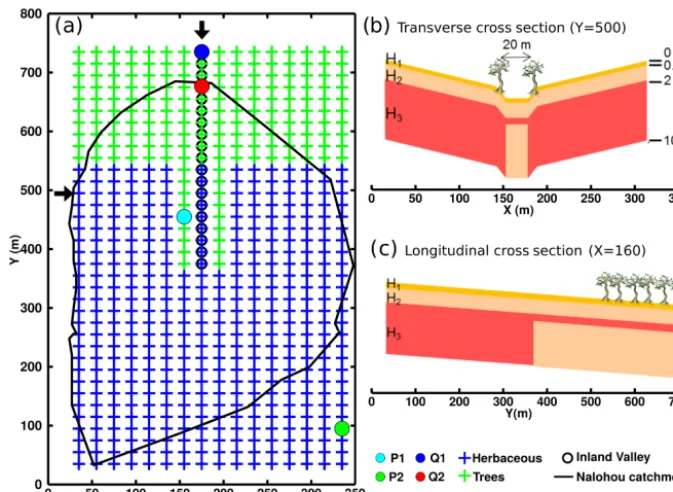
In this section, we briefly describe our conceptual repre-sentation of the main soil and vegetation characteristics found in the hard-rock basement areas of the Sudanian cli-matic region (yearly precipitation amount between 700 and 1400 mm) dominated by metamorphic settings. This eco-physical model is built following the literature of the region and on inland valleys and the work of Hector et al. (2015), who studied and described the functioning of an elemen-tary catchment in northern Benin, the Nalohou catchment (0.16 km2). This catchment is part of the regional AMMA-CATCH observatory, which belongs to the OZCAR network of critical zone observatories (Gaillardet et al., 2018). See for instance Fig. 13 in Hector et al. (2015) for a concep-tual sketch of their understanding of the Nalohou catchment: during the dry season the permanent water table is discon-nected from the inland valley, while during the wet season, the permanent water table rises and a shallow perched wa-ter table appears in the inland valley which is fed by both rainwater infiltration and lateral subsurface transfers. This specific behaviour is representative of inland valley function-ing in similar geological/climatic contexts (see e.g. Brabant, 1991, in Cameroon, Diatta, 1996, in Ivory Coast or Giertz and Diekkrüger, 2003, in the other location in Benin). In the Nalohou case, lateral subsurface contributions to the inland valley differ from each bank: contributions from the layered left bank (highly permeable hardpan over low-permeability clay-rich horizons) exceed contributions from the sandier right bank. Figure 1a shows the actual catchment shape as a black line and cross sections of Fig. 1b–c summarize the internal structure of the catchment.

2.1.1 Soil layers and properties

Our conceptual model of the physical environment is made up of three layers through depth (H1: 0–0.5, H2: 0.5–2, H3: 2–10.5 m, Fig. 1b–c), to which we prescribed specific hydro-dynamic properties in a deterministic way and following the literature, but is also based on numerous field and laboratory measurements by Hector (2014), Richard (2014) and Robert (2012) in the same area (Table 1). In the following text, we refer to sand-like and clay-like hydrodynamic properties in a broad sense: sand-like relates to highly permeable/low-retention media and clay-like relates to low-permeable/high-retention media. The reader may refer to Tables 1 and 3 for actual property ranges and values.

The thicknesses of the two shallowest soil layers (H1 and H2) are well defined from observations in the Nalohou catchment, and seem in accordance with other locations in

(sub)tropical humid regions (de Condappa et al., 2008). The thickness of the deeper layer (H3) is that of the regolith, lo-cated above the fissured basement and the hard-rock base-ment, following Lachassagne et al. (2011).

Layer H1

In the tropical-humid Sudanian climate, topsoils are usu-ally permeable, due to microfauna bioturbation or soil work from farmers (Giertz and Diekkrüger, 2003; Richard, 2012; Robert, 2012). As a consequence, the infiltration-excess overland flow is very limited in the area (e.g. Giertz et al., 2006; Masiyandima et al., 2003). The topsoil layer, H1, is therefore permeable, with sand-like soil hydrodynamic prop-erties. Some authors note a significant relationship between saturated hydraulic conductivity and land cover in the area (Giertz et al., 2005; Giertz and Diekkrüger, 2003; Richard, 2014), but in a limited range (less than 1 order of magni-tude). The H1 layer is thus considered laterally homogeneous in this study.

Layer H2

The second layer (H2) is usually more variable laterally, and variations in clay content in this potential illuviation layer (a clay-accumulation horizon, as described by de Condappa et al., 2008) may generate perched water tables (e.g. Giertz et al., 2006). In this layer, some macroporous hardpan units with high permeability may also be found (Bonsor et al., 2014; Hector et al., 2015).

It is beyond the scope of this study to analyse the ef-fect of this layer (H2) on the hydrological processes. There is an extensive literature using the same critical zone mod-elling framework that provides insights into the effect of lat-eral variability of soil properties through dedicated sensi-tivity studies (Atchley and Maxwell, 2011; Meyerhoff and Maxwell, 2011; Meyerhoff et al., 2014; Gilbert et al., 2016). We therefore chose to consider a rather sandy, permeable layer to mimic a hardpan unit behaviour (as part of the poly-cyclic soil profile described by Faure and Volkoff, 1998), and favour quick lateral subsurface transfer, which has been ob-served in the area (e.g. Hector et al., 2015; Masiyandima et al., 2003 and Séguis et al., 2011).

Layer H3

Figure 1. (a)Catchment mesh. Blue and green crosses indicate the vegetation distribution for the reference case. Inland valley cells are shown as black circles.P are water table sampling locations andQare streamflow sampling locations.(b, c)Domain cross sections schematically made up of three soil types: high-permeability sandy soils (yellow), hardpan or fissured basement (orange) and low-permeability clay accu-mulation (red).

Nalohou catchment, and is the second major feature from larger-scale observations by Faure and Volkoff (1998). Inland valley

The inland valley is located in the downstream part of the valley thalweg (circles of Fig. 1a). It has a specific H1/H2/H3 sequence. It usually consists of sandy upper horizons. H1 and H2 layers are the same as elsewhere, and are considered to be of a sandy nature and to favour quick vertical and lateral transfers, as observed in the field. At about 2 m depth, in the upper part of the H3 layer just below the H2 horizon, is a low-permeability, clayey layer, which actually characterizes the inland valley. This allows the formation of perched water tables during the rainy season (Masiyandima et al., 2003). Such a shallow drainage system is the main contributor to baseflow, which represents roughly 80 % of total streamflow for such a catchment (Giertz et al., 2006; Hector et al., 2015; Kamagaté et al., 2007; Séguis et al., 2011). This clay-rich ac-cumulation horizon is often found above a poorly weathered horizon (Brabant, 1991), as is the case in the Nalohou catch-ment. Therefore the H3 layer underneath the inland valley is made of a low-retention, high-permeability fissured base-ment (in the sense of Lachassagne et al., 2011).

Hydrodynamic properties

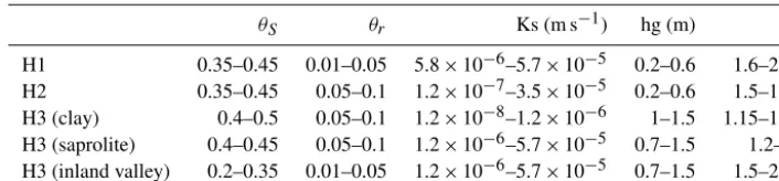
In a thesis work, Hector (2014) summarized the variability of field measurements to build up classes of main soil/lithology units for the three main layers identified in this study (Ta-ble 1). Hydrodynamic parameters (following Van Genuchten, 1980) for this study are shown below in Table 3. Satu-rated conductivities of saprolite and fissured basement in H3 are given by the range of observations derived from both pumping tests and magnetic resonance soundings in the area (Vouillamoz et al., 2014).

2.1.2 Topography

lateral-Table 1.Ranges of hydrodynamic properties in the area, following Van Genuchten (1980). From Hector (2014).

θS θr Ks (m s−1) hg (m) n

H1 0.35–0.45 0.01–0.05 5.8×10−6–5.7×10−5 0.2–0.6 1.6–2.2 H2 0.35–0.45 0.05–0.1 1.2×10−7–3.5×10−5 0.2–0.6 1.5–1.8 H3 (clay) 0.4–0.5 0.05–0.1 1.2×10−8–1.2×10−6 1–1.5 1.15–1.5 H3 (saprolite) 0.4–0.45 0.05–0.1 1.2×10−6–5.7×10−5 0.7–1.5 1.2–2 H3 (inland valley) 0.2–0.35 0.01–0.05 1.2×10−6–5.7×10−5 0.7–1.5 1.5–2.2

resolution DEM derived from the DGPS survey, as described in Hector et al. (2013).

2.1.3 Vegetation

Non-disturbed natural vegetation in this area is mostly wood-land, composed of trees with a herbaceous layer underneath. Under human influences, trees are usually cut in favour of agricultural plots. However, trees in the riparian areas and the inland valley fringes are generally kept alive, as well as specific species on the hillslopes for consumption pur-poses (agroforestry system). This is why we consider in this study two vegetation classes: trees and herbaceous. While the trees class refers to a fully tree-covered state with some herbaceous layer underneath, the herbaceous cover refers to a mixed fallow-field landscape with sparse trees, composed of either cultivated plots or young fallows under the influence of farmers or with some isolated trees (with height<10 m) kept for local consumption.

Tree phenology mostly consists in defoliation around Jan-uary, which occurs asynchronously between different species and different individuals of the same species (Seghieri et al., 2012). On the other hand, in the so-called herbaceous cover, the ground is commonly covered by scattered shrubs, while the actual herbaceous layer usually starts growing in April after the first rains and reaches its maximum height (up to 2.5 m) in October. At this time its height exceeds that of shrubs. Then, the herbaceous layer stops transpiring and dries up from October to January. Controlled fire is a traditional practice in Benin; the vegetation (mainly the herbaceous layer) is burnt between November and February. Hence, dur-ing the dry season, the soil is bare for about 5 months. Leaf area index (LAI) and stem area index of trees and herbaceous classes are later shown in Fig. 6a.

2.2 Critical zone model

The CZ model ParFlow-CLM (PFCLM) is composed of ParFlow, a three-dimensional integrated physical model that simultaneously solves variably saturated flow and surface outflow coupled with CLM, a land surface model which solves both the water and energy budget at the surface. ParFlow uses a free-surface overland flow boundary condi-tion which routes ponded water as overland flow using the kinematic wave equation and Manning equation (Kollet and

Maxwell, 2006). In this study, the topographic effect is taken into account by a terrain-following grid (Maxwell, 2013) and only requires two-dimensional surface slopes to be provided. ParFlow solves the Richards equation using cell-centered fi-nite differences in space and an implicit backwards Euler scheme in time. The Newton–Krylov method is used together with a multigrid preconditioner and shows excellent parallel scaling, which allows the simulation of large-scale domains (i.e. continental US) at high resolution (i.e.<1 km) (Ashby and Falgout, 1996; Jones and Woodward, 2001; Maxwell et al., 2015). ParFlow is coupled through the user-definedN -first cells from the surface to a modified version of the Com-munity Land Model (CLM) which solves both the water and energy budget at the surface (Dai et al., 2003; Maxwell and Miller, 2005). CLM has one vegetation layer and the ver-sion within ParFlow currently only allows a single vegeta-tion class per surface grid cell. PFCLM is an excellent can-didate for this study because it allows the representation of a number of physical processes that have been observed in Sudanian western Africa (perched water tables, groundwa-ter and subsurface wagroundwa-ter baseflow, stormflow, plant transpi-ration and bare ground evapotranspi-ration). This is achieved us-ing physical parameters (hydrodynamic properties, vegeta-tion parameters, complex three-dimensional lithological or pedological units) and without prior specification of the pro-cesses. The model has already been successfully applied in the region, using measured parameters for simulating vertical water fluxes (evapotranspiration, percolation) and specific features like perched water tables (Robert, 2012). We used the tagged version v3.3.1-IGE (https://github.com/ basileh/parflow/releases/tag/v3.3.1-IGE, last access: 24 Oc-tober 2018).

2.3 Model set-up

We model an idealized elementary headwater catchment, comprising an inland valley, of 720 m×300 m catchment (0.216 km2), with a 20 m lateral (x, y) resolution (Fig. 1, Ta-ble 2). The idealized inland valley and its contributive area have a V-shaped type (Maxwell et al., 2014), sloping in the

Y direction (Fig. 1a). TheY direction slope is 4 % and theX

Table 2.Model set-up

Property Value

Extension X 300 m Extension Y 720 m Extension Z 10.5 m DX (grid resolution) 20 m

DY 20 m

DZ variable: 0.13–1.19 m Duration 8 years

Dt 0.5 h

Slope X 2 %

Slope Y 4 %

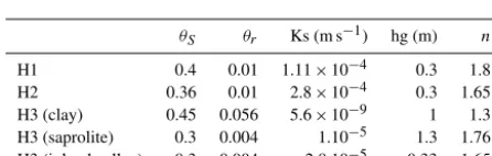
Table 3.Hydrodynamic properties for the virtual V-shaped catch-ment, following Van Genuchten (1980).

θS θr Ks (m s−1) hg (m) n

H1 0.4 0.01 1.11×10−4 0.3 1.8

H2 0.36 0.01 2.8×10−4 0.3 1.65

H3 (clay) 0.45 0.056 5.6×10−9 _{1 1.3} H3 (saprolite) 0.3 0.004 1.10−5 1.3 1.76 H3 (inland valley) 0.3 0.004 2.8.10−5 0.33 1.65

These cells are further lowered by 2 m below the altitude of the inland valley fringes, to represent the classically observed banks.

The vertical resolution varies with depth following a geo-metric progression of common ratio 1.2 for the first 13 cells (which are coupled to CLM), ranging between 0.134 and 1.195 m, and 4 more 1 m thick cells, uncoupled to CLM, are added at the bottom. The domain is therefore 10.5 m thick. Selected hydrodynamic parameters based on expertise-driven sensitivity studies within the range of observed values (Table 1) are shown in Table 3.

No-flow boundary conditions are applied to the catchment edges (symmetric assumption) and bottom. The only way for the water to leave the domain, apart from evapotranspiration, is through overland flow at the catchment outlet.

2.4 Model forcings 2.4.1 Atmospheric forcing

Forcing data are obtained from the Benin site of the AMMA-CATCH observatory (AMMA-AMMA-CATCH, 1996) and are avail-able on the data portal (http://db.amma-catch.org, last ac-cess: 24 October 2018). This meso-scale site comprises the Upper Ouémé catchment (14 300 km2) which is representa-tive of the Sudanian climate. The meteorological variables used to force CLM (wind speed, air temperature and hu-midity, pressure and the incoming radiative long and short waves, Fig. 2) were measured at a 2 m height on a flux tower located on a cultivated site (the Nalohou catchment,

lat. 9.74◦N, long. 1.60◦E, 449 m a.s.l.). Rainfall is measured with a tipping-bucket rain gauge.

Western African rainfall follows the monsoon dynamics and is characterized by a strong variability at interannual scales (see e.g. Lawin (2007) and Le Lay and Galle (2005) for detailed analyses of the Sudanian rainfall regime). In the simulated years, yearly precipitation amounts ranged from 913 to 1572 mm (Fig. 2).

Figure 2 shows the meteorological variables used to force PFCLM. They have been described in Mamadou et al. (2014) for the year 2008 and recently compared to data from a site 13 km away over a forested cover for the period 2008–2010 (Mamadou et al., 2016). The daily meteorological conditions of the two sites were expectedly close. Minimal values of incoming short-wave radiations (SWin) are observed during

the wet season due to cloud cover, and low values are also found at the core of the dry season, due to aerosols brought by the north-easterly Harmattan winds. Incoming long-wave radiations (LWin) are low during the dry season due to the

re-duced cloud cover. The highest air temperatures are observed before the start of the wet season, while the wet season ex-hibits the lowest daily average and amplitude of temperature. Specific humidity clearly shows the monsoon/Harmattan sig-nal: during the wet season, moist air is brought by the south-westerly to southerly monsoon winds and during the dry sea-son north-easterly Harmattan winds bring dry air from the Sahara. The Harmattan blows as a light to moderate breeze. These weather types are typical for Sudanian regions (Lohou et al., 2010; Sultan and Janicot, 2003).

PFCLM is forced at a 30 mn time step, over the 7-year pe-riod 2006–2012, with spatially homogeneous forcings. Initial conditions are set as a water table depth of 3 m, in accordance with several water table measurements. The model is spun up for 1 year, which corresponds to the year 2007, a rather aver-age year.

2.4.2 Vegetation forcings

In this study, we forced the model with observation-based time series of LAI, SAI (stem area index), displacement heights and roughness lengths for the two vegetation classes of our domain (trees and herbaceous).

10 30 50 70

Precip (mm)

0 400 800

SWi (W

m

)

0 400 800

LWi (W

m

)

10 20 30

Tair (°C)

0.005 0.010 0.015

SH (kg kg )

2005 2006 2007 2008 2009 2010 2011 2012

0 2 4 6 8

Wspeed (m s )

-1

-1

-2

-2

Figure 2.Model forcing. Upper panel: daily precipitation. SWin: incoming short waves, LWin: incoming long waves,Ta: air temperature,

SH: specific humidity, wind spd: wind speed. Data are shown as the daily mean (black curve) and daily minima and maxima (shaded area).

MODIS, SEVIRI), constrained by in situ measurements de-rived from hemispherical photographs based on the method proposed by Weiss et al. (2004), on both the forested and herbaceous-covered sites. Herbaceous SAI is also calculated from LAI using the equation (LAI+SAI=LAImax) during

the senescence period (see the later Fig. 6a for the LAI and SAI time series used in the model forcing).

For the herbaceous cover, the root distribution in the model follows that of Zeng (2001), which is an exponential shape for the cumulative root fraction (Y) to depth (d) of equation

Y =1−1

2(e

−ad_+e−bd_{), with the two coefficientsa=9 and} b=2. For the trees, the distribution is kept uniform over the first 3 m below the surface, because we found the Zeng equation not relevant for most Sudanian trees for which ef-ficient deep roots have been observed (Jourdan, Gnanglé, Seghieri and Peugeot, personal communication). The clos-est published study on deep roots in natural forclos-est is in a slightly different setting in tropical semi-deciduous rain for-est where 95 % of all roots from E. cylindricum were dis-tributed to depths of between 2.58 and 5.64 m (Freycon et al., 2015).

2.5 Evaluation data

As a first step, we evaluate the relevance of the model with respect to real-world data (water table depth measurements, soil moisture, streamflow records, evapotranspiration and gravity data). This section describes the evaluation data ob-tained from the Nalohou catchment, whose size and struc-ture are comparable to that of our virtual V-shaped catch-ment (Fig. 1a). The Nalohou catchcatch-ment comprises a small inland valley and is considered to be representative of a cul-tivated site. It has been the focus of previous studies

(De-scloitres et al., 2011; Guyot et al., 2012; Hector et al., 2015; Richard et al., 2013). Land surface elevation ranges from 436 to 460 m.a.s.l., and topographic slopes are gentle (mean N–S and E–W slopes correspond to those imposed on the virtual V-shaped catchment).

Observations in P1 and P2 (Fig. 1a) were used to evaluate the simulated groundwater dynamics. At the inland valley lo-cation in P1 there is a shallow, 1 m deep piezometer which aims at documenting the seasonal perched water table and a deeper (10 m) piezometer monitoring the permanent water table.

Streamflow measurements have been described in AMMA-CATCH (2008). A Parshall flume was built in 2004 at the outlet of the inland valley (Q2 in Fig. 1a) and recorded any level change above 10−3m, using a level probe (OTT Thalimedes).

Two eddy covariance flux towers have been installed, re-spectively, on the Nalohou site (where the flux tower foot-print is representative of cultivated, herbaceous-like areas) and on the woodland site (Mamadou et al., 2016). Further-more, an infrared large-aperture scintillometer (LAS) was deployed from 2006 to 2008 on the Nalohou site (Guyot et al., 2009, 2012). LAS measurements give access to an aver-age sensible heat flux over the footprint area and, by closing the energy budget, this allows us to derive the average latent heat flux (i.e. evapotranspiration). On the Nalohou site, the beam path was 2.4 km long, and comprised many more trees than in the flux tower footprint area.

moisture content is derived from the measurements at a hourly time step (AMMA-CATCH, 2005b).

Gravity instrumentation originates from the GHYRAF (Gravity and Hydrology in Africa) project, which sought to study gravity to water storage change (WSC) relationships (Hinderer et al., 2009, 2012). Gravity instruments were an absolute (AG hereafter) FG5 gravimeter (Hector et al., 2013), a relative superconducting gravimeter (Hector et al., 2014, SG hereafter) and a CG5 relative portable spring gravimeter (Hector et al., 2015). Relative spring microgravimeters mea-sure differences in gravity between stations, while other in-struments such as SG or AG measure changes at a specific site. Hybrid gravimetry is the joint use of gravity surveys using relative microgravimeters and monitoring of temporal changes at a base station, using an SG and/or AG (Hinderer et al., 2016). From the hybrid gravity data set of Nalohou, Hec-tor et al. (2015) produced a map of the seasonal amplitude of gravity changes (their Fig. 11). In this study, we convert grav-ity changes to water storage changes using a simple scalar ad-mittance (gravity changes to WSC ratio) of 0.04 µGal mm−1, in accordance with local topography, and following the ad-mittance calculated by Hector et al. (2015).

2.6 Analysis tools

WSC analysis is conducted using empirical orthogonal func-tion (EOF) decomposifunc-tion. EOF decomposifunc-tions can be seen as principal component analysis applied to the time series of a spatial field. The method produces spatial patterns of vari-ability (in terms of variance), their associated time variation together with a measure of the weight (importance) of each pattern (in terms of explained variance). In other words, the whole data set of coordinates (x, y, t) is decomposed into the weighted sum of modes, where each mode is the product of an EOF spatial pattern (an (x, y) map) with a normalized time series. The weights are given in terms of how much of the to-tal signal variance is contained in the associated mode. This method has been used on WSCs from hybrid gravity data and neutron probe data at the Nalohou catchment size by Hector et al. (2015), who showed that the first mode could be inter-preted as the seasonal signal.

To measure the goodness-of-fit between simulations and observations, we use the Kling–Gupta efficiency (KGE) cri-terion (Gupta et al., 2009):

KGE=1−

q

(r−1)2+(α−1)2+(β−1)2, (1) where r is the linear correlation coefficient between simu-lated and observed time series and

α= σS

σO

;β= µS

µO

, (2)

and(µS, σS)and(µO, σO)are the mean and SD of,

respec-tively, simulated and observed time series. KGE has an ideal value at unity.

2.7 Overview of the three virtual experiments

We model an elementary headwater catchment and test its sensitivity to (1) the presence of a low-permeability layer un-derneath an inland valley, (2) the vegetation distribution, and (3) the hydrodynamic properties of contributive areas (H3 layer). To do so, we build a set of virtual experiments that are compared to a benchmark simulation (named the “reference” case hereinafter, Table 4). This reference simulation includes an inland valley characterized by an impervious layer made up of a clay lens underlying an upper sandy layer in the val-ley thalweg. Vegetation distribution and H3 layer are both chosen arbitrarily in this simulation. An anthropized vege-tation distribution (mostly herbaceous but also with trees in the riparian areas) allows comparison of model outputs with observed hydrological variables at the Nalohou catchment. A clay-like contributive area (H3 outside the inland valley cells) is chosen between the two main pedological features (clay and saprolite). The three virtual experiments are as fol-lows (Table 4).

The first experiment explores the impacts of the low-permeability layer in the valley thalweg on the hydrological functioning of the catchment. This experiment consists in re-moving the impervious layer below the H2 horizon (upper part of H3 as shown in Fig. 1b) in the valley thalweg with re-spect to the reference case. Other parameters (hydrodynamic, vegetation) are kept identical.

The second experiment explores the impact of the vege-tation cover with three cases: the “natural” state where the catchment is fully covered with trees, and the “anthropized” state with two different vegetation covers: (1) either the catchment is covered with grass, except in the riparian and inland valley fringe areas where trees remain (as in Fig. 1a – this is the reference case), or (2) the catchment is fully cov-ered with grass (no trees).

Table 4.Virtual experiments. “Trees and herbaceous” refers to trees only in riparian areas and inland valley fringes, as shown in Fig. 1.

Clay lens in H3 layer Vegetation the valley thalweg

Reference case yes Clay Trees and herbaceous

Exp. 1: inland valley no Clay Trees and herbaceous

Exp. 2: vegetation yes Clay Trees only

Herbaceous only

Exp. 3: contributive areas yes Saprolite Trees and herbaceous

Clay in the west, saprolite in the east

3 Results

3.1 Reference case and saprolite case compared to Nalohou observations

3.1.1 Water storage changes

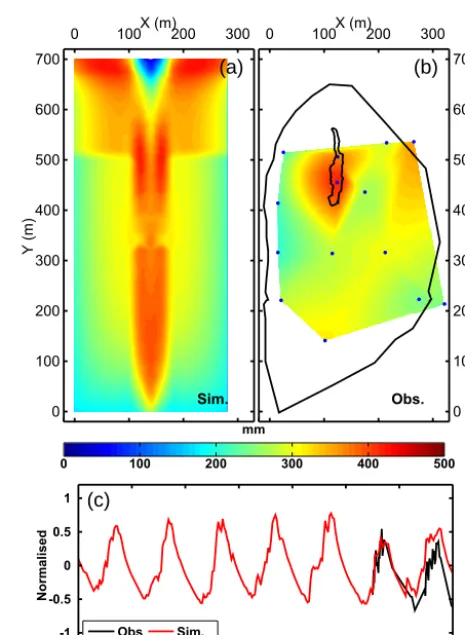
Water storage changes (WSCs) are shown in Fig. 3 as the spatial and temporal patterns of the first mode of the EOF decomposition. While the left panel shows the simulated WSCs, the right panel shows WSCs obtained from the hy-brid gravity data by interpolation from point-based values (blue dots). The first mode of the simulated WSCs repre-sents more than 90 % of the variance. This means that more than 90 % of the total signal variance is contained in the first EOF spatial pattern multiplied by its associated time series (Fig. 3c, red line). The time series shows that this mode cor-responds to the seasonal cycle (the common part of the signal which explains most of the total variance). In that sense, we can directly interpret the spatial patterns (i.e. the EOFs) as maps of seasonal water storage amplitudes. The first mode of gravity-derived WSCs also explains a significant part (79 %) of the total variance. As this map derives from an interpo-lated field, and although gravity data are spatially integrative, observed geometries should not be overinterpreted. Mode 2 (not shown) accounts for about 8 % of the total variance, and contains interannual storage variations together with some residuals at the seasonal level.

The reference simulation includes an inland valley (a low-permeability layer in the upper part of the H3 horizon) and the clayey material in the H3 layer outside the inland val-ley corresponds to what is found on the western bank of the Nalohou catchment. In this regard, the simulated spatial pat-tern matches two important features of the observations: a high amplitude in the inland valley and a low amplitude in the clayey area. The high simulated amplitude in the down-stream section (500 to 700 m) is due to tree withdrawals dur-ing the dry season. Gravity data do not cover this part of the catchment, which prevents the comparison with the

sim-Sim. X (m)

Y (m)

0 100 200 300

0 100 200 300 400 500 600 700

Obs. X (m)

Y (m)

0 100 200 300

0 100 200 300 400 500 600 700

mm

0 100 200 300 400 500

Normalised

2005 2006 2007 2008 2009 2010 2011

-1 -0.5 0 0.5 1

Obs Sim.

(a) (b)

(c)

Figure 3.Empirical orthogonal function decomposition of water storage changes (WSC).(a, b)Spatial patterns of WSC for the first mode of EOF.(a)Simulated WSC and(b)observed, gravity-derived WSC at the Nalohou catchment (blue points are station locations). The outline of the inland valley is shown for the Nalohou catchment. (c)Temporal pattern of the first mode of simulated and observed WSC.

transfer to the valley thalweg where water accumulates dur-ing the wet season, and drains down toward the riparian areas during the dry season. High amplitude is simulated along the whole valley thalweg and not only in the inland valley, as the observation shows.

3.1.2 Water table

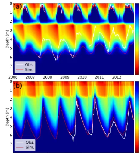
Figure 4a shows simulated time series of saturation profiles at P1, in the inland valley for the reference simulation. Red lines show the simulated water tables, while white lines show the observed water tables. The model is able to reproduce seasonal fluctuations of both the permanent water table and the temporary perched water table. Although numerous dis-crepancies exist (e.g. the seasonal amplitudes of the perma-nent water table), mainly because of the horizontal and verti-cal variability of hydrodynamic parameters which have been considered constant in layer H3, the first order of this com-plex behaviour is reproduced. In particular, the interannual behaviour of the permanent water table is rather satisfying, despite a slight phase shift, but higher-frequency responses of the shallow perched water table at the core of the rainy season are also well reproduced.

Figure 4b shows simulated time series of saturation pro-files at P2, in the upstream area for the saprolite simulation (sandy H3 layer everywhere but in the inland valley). This sandy H3 layer is a common feature of the environment, par-ticularly on the eastern bank of the Nalohou catchment. The simulated permanent water table matches satisfyingly the ob-servation representative of this sandy H3 unit.

3.1.3 Streamflow

Figure 5 shows simulated and observed streamflow ex-pressed in mm h−1, which allows the comparison between the Nalohou catchment (0.16 km2) and the V-shaped model (0.22 km2). We chose to focus the plot on the baseflow part of the time series, cutting the highest flow peaks, for two reasons: (1) Hector et al. (2015) noted that in such settings baseflow is the major contributor to total measured stream-flow (about 80 %) and (2) the following sections will present semilog plots of the different experiments simulated, which allow us to display the whole range of streamflow values but with less intuitive interpretation. Overall, the match is sat-isfying, and the simulation respects baseflow onset and re-cession behaviours. The only negative KGE value for the year 2009 composed of (r=0.96, α=1.56, β=1.84) is mostly explained by a high bias and overly high simulated variance, while the time phasing matches well. It has to be noted that the simulation produces higher flow peaks than observed for some events, but not all (see further Fig. 9). Discrepancies between observed and simulated streamflow are higher in drier years (i.e. 2011). This is due to the plexity of connectivity between different contributive com-partments, which is over-simplified in our idealized

simula-Figure 4.Simulated saturation and observed and simulated water table.(a)In the inland valley (at P1) and for the reference simula-tion (clayey H3 layer);(b)in the upstream area (at P2) and for the saprolite simulation (sandy H3 layer).

tion. The simulated diurnal cycle in the ponded water (from which streamflow is calculated) is a model artifact due to the ponded cell size (20 m wide here).

3.1.4 Evapotranspiration

Figure 6a shows the LAI and SAI forcing time series used in this study for the two vegetation covers. Figure 6b (or Fig. 6d) shows the simulated daily evapotranspiration spa-tially averaged over herbaceous-covered cells out of the thal-weg in light blue line for the reference simulation (or the saprolite simulation). The shaded area gives the whole spa-tial range of daily values between minimal (lower black line) and maximal (upper black line) spatial evapotranspiration. Figure 6c (or Fig. 6e) is similar, but for tree-covered cells. Reference (clay in the H3 unit everywhere but below the in-land valley) and saprolite simulations are compared because the Nalohou flux tower is located on a saprolite-like mate-rial. The saprolite simulation actually matches more closely the observed evapotranspiration in the dry season.

abil-Jul Aug Sep Oct Nov 0.0

0.3 0.6

-1

r2_{= 0.64}

KGE = 0.65

2008

Obs. Sim.

Jul Aug Sep Oct Nov

0.0 0.3

0.6 r

2_{= 0.92}

KGE = -0.01

2009

Jul Aug Sep Oct Nov

0.0 0.3 0.6

mm h

r2_{= 0.91}

KGE = 0.82

2010

Jul Aug Sep Oct Nov

0.0 0.3

0.6 r

2_{= 0.28}

KGE = 0.28

2011

Jul Aug Sep Oct Nov

0.0 0.3

0.6 r_{KGE = 0.84}2= 0.80

2012

-1

mm h

-1

mm h

-1

mm h

-1

mm h

Figure 5.Observed and simulated streamflow for the wet seasons of the period 2008 to 2012 at station Q2.

ity to transpire with a higher LAI. During the wet season, the evapotranspiration is never water limited (Mamadou et al., 2016). During the transition period between wet and dry seasons, the herbaceous layer dries up, and LAI is replaced by SAI, which diminishes drastically the evapotranspiration. Herbaceous are eventually burnt at the end of this transition period (SAI drop in Fig. 6a), while trees start renewing their leaves.

Overall, the spatially averaged simulated evapotranspira-tion matches the observaevapotranspira-tions, over both herbaceous and tree covers. At the end of the wet season, the simulated evapo-transpiration (dominated by evapo-transpiration) is a little higher than the EC observations, but not higher than the LAS obser-vations in 2008. EC is known to underestimate evapotranspi-ration (Foken, 2008).

3.1.5 Soil moisture

Because soil moisture probes are located on the eastern side of the Nalohou catchment, observed soil moisture is here compared to the “saprolite” simulation where H3 outside the inland valley is composed of sandy-like saprolite (Fig. 7). Simulations match the observed temporal patterns in a satis-fying way, including recession behaviours.

3.1.6 Annual water budget

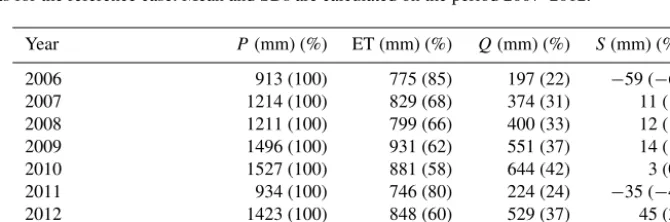
The water budget simulated for the reference case is shown in Table 5. As expected, evapotranspiration dominates the water budget (from 58 % to 83 % of the yearly precipitation amount) but shows a marked interannual variability as sim-ulated in the area at basin scale (Cornelissen et al., 2013; Séguis et al., 2011) and from a review of different other spa-tial scales (Hector, 2014). For dry years, the ET part (or theQ

part) of the budget is higher (or lower) than for wet years. In-terannual water storage changes are rather limited and do not seem to exhibit memory effects. In other words, the relative part of (ET+Q) in the water budget is stable over years. If we now consider the absolute values of the water balance terms, the difference between a wet year (2010) and the following dry year (2011) is 593 mm in rainfall, 135 mm in evapotran-spiration, 420 mm in streamflow and 38 mm in water storage. Streamflow is the most affected term in a dry year: it under-goes a drastic loss of water, about 3 times greater than that of evapotranspiration, almost equal to its interannual average (454 mm). This results in the interannual SD ofQbeing more than twice as large as the standard deviation of ET: the inter-annual variability in precipitation (SD=225 mm) is mostly compensated by streamflow (151 mm) and to a lesser extent by evapotranspiration (64 mm) and water storage changes (26 mm).

3.2 Virtual experiments

3.2.1 Annual water budgets

0 2 4

Index

(a) LAI herbaceous LAI trees SAI herbaceous SAI trees

0 2 4

6 Sim (ref): herbaceous Obs: EC Obs: LAS (b)

0 2 4

6 Sim (ref): trees Obs: EC Obs: LAS (c)

0 2 4

6 Sim (saprolite): herbaceous Obs: EC Obs: LAS (d)

0 2 4

6 Sim (saprolite): trees Obs: EC Obs: LAS (e)

2006-010 2006-07 2007-01 2007-07 2008-01 2008-07 2009-01 2009-07 2010-01 2010-07 25

50 75

mm d

(f) Precipitation

-1

mm d

-1

mm d

-1

mm d

-1

mm d

-1

Figure 6. (a)LAI and SAI forcings for tree and herbaceous covers.(b–e)Observed and simulated evapotranspiration over herbaceous cells (b)and tree cells(c)for the reference simulation and the saprolite simulation (dande). Blue line shows the spatial average over all cells of the respective cover out of the inland valley, and the shaded area shows the extent of spatial maxima and minima.(f)Precipitation.

Table 5.Water budgets for the reference case. Mean and SDs are calculated on the period 2007–2012.

Year P (mm) (%) ET (mm) (%) Q(mm) (%) S(mm) (%)

2006 913 (100) 775 (85) 197 (22) −59 (−6)

2007 1214 (100) 829 (68) 374 (31) 11 (1)

2008 1211 (100) 799 (66) 400 (33) 12 (1)

2009 1496 (100) 931 (62) 551 (37) 14 (1)

2010 1527 (100) 881 (58) 644 (42) 3 (0)

2011 934 (100) 746 (80) 224 (24) −35 (−4)

2012 1423 (100) 848 (60) 529 (37) 45 (3)

Mean±SD (2007–2012) 1301±225 839±64 454±151 8±26

during the dry years. This results in a higher interannual SD of the storage term.

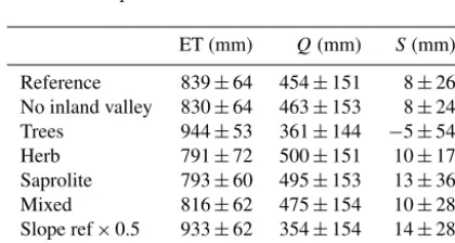
The presence of the impermeable layer (in the reference case) has very little effect on the water budget, lowering the streamflow by 2 % (9 mm) on average, in favour of evapo-transpiration, with respect to the case without the imperme-able layer.

0.0 0.1 0.2 0.3

m

3

m

-3

Obs: 5 cm Sim: 7 cm

0.0 0.1 0.2 0.3

m

3

m

-3

Obs: 10 cm Sim: 7 cm

0.0 0.1 0.2 0.3

m

3

m

-3

Obs: 20 cm Sim: 21 cm

2006 2007 2008 2009 2010 2011 2012

0 25 50 75

mm d

Precipitation

-1

Figure 7.Observed and simulated soil moisture for the saprolite simulation at location P2.

Table 6.Interannual mean and SD of simulated evapotranspiration (ET), streamflow (Q) and storage (S) for the different virtual exper-iments and for the period 2007–2012.

ET (mm) Q(mm) S(mm)

Reference 839±64 454±151 8±26 No inland valley 830±64 463±153 8±24 Trees 944±53 361±144 −5±54 Herb 791±72 500±151 10±17 Saprolite 793±60 495±153 13±36 Mixed 816±62 475±154 10±28 Slope ref×0.5 933±62 354±154 14±28 Slope ref×2 773±64 526±157 1±21

3.2.2 Water storage

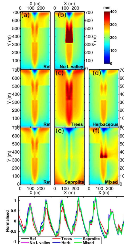
Figure 8 shows water storage changes as the first modes of the EOF decompositions for all tested cases. In all cases, the first mode represents more than 90 % of the variance.

The most striking discrepancies arise when comparing the results related to the contributive area experiments (Fig. 8a, e, f). While the reference case (clayey H3 layer, Fig. 8a) shows low seasonal amplitude in the valley banks and higher amplitude along the valley axis including the in-land valley, the saprolite case (Fig. 8e) shows a rather oppo-site behaviour with higher amplitude on the banks and lower amplitude in the valley axis. In the reference case, the south-ern, upstream edge of the inland valley exhibits a break in the

seasonal amplitude, while this is not visible in the saprolite case (in this case there is no specific imprint of the inland val-ley). In the mixed case (Fig. 8f), the southern, upstream edge of the inland valley also exhibits a different seasonal ampli-tude, but of opposite behaviour, as in the reference case.

In the vegetation experiment (Fig. 8a, c, d), the tree-covered catchment (Fig. 8c) shows higher seasonal ampli-tude than the herbaceous-covered catchment (Fig. 8d), while the reference case shows patterns closer to the herbaceous-covered catchment. In the time series, seasonal WSC in-crease occurs earlier on herbaceous cover than on trees.

The absence of the impermeable layer in the inland val-ley increases the seasonal water storage amplitude along the thalweg (Fig. 8b).

In all cases, there is low seasonal amplitude at the catch-ment outlet (the northern blue patch). This is the imprint of the topography (all cells converge to that point) and the model boundary condition: the only way for the water to exit the domain, apart from evapotranspiration, is through this outlet.

descrip-tive model), while streamflow, evapotranspiration and spatial pattern of WSC are well reproduced, the simulated perma-nent water table completely fills up the inland valley due to high permeability in the H3 layer on the right bank (see fur-ther), which is not observed. Hence there must be some bar-rier to the lateral flow feeding the inland valley. However, it would be interesting to investigate the existence of other in-land valleys which do not show such disconnexion between the upper perched water table and lower permanent water ta-ble. Our study would anticipate that, all scaling issues dis-carded, such an inland valley would produce a similar water budget.

3.2.3 Streamflow

Yearly simulated streamflow time series (sampled on cell Q1, Fig. 1) are shown in Fig. 9 for the year 2011 and as semilog plots, with the reference time series repeated in all plots in black. Overall, streamflow simulations are rather similar. Many of the differences among the cases are related to the first part of the rainy season, in the timing of the stream-flow onset and the streamstream-flow amplitude during this period (this is also true for other years, not shown). Differences in the dry season are very low in terms of water amount (cf. the log scale), but exhibit clearly different behaviours: some cases are able to sustain a low baseflow during the dry sea-son, while some others, including the reference case, prevent water flow during the dry season.

The presence of the impermeable layer in the inland val-ley (reference case) induces a higher streamflow in August (Fig. 9a). On the other hand, the absence of the impermeable layer favours infiltration and maintains a low baseflow longer in the dry season, fed by the permanent water table which is then connected all across the catchment.

The tree-covered catchment (Fig. 9b) tends to exhibit lower streamflow in August. The storm peaks are much at-tenuated, as compared to the reference case. The herbaceous-covered catchment shows a higher streamflow in the dry season and the early wet season, with slightly higher storm peaks than in the reference case. One may note how the refer-enceQfollows the treesQin the early season before August and then migrates to meet the herbaceousQthat it follows until the reverse migration is observed in November. This likely denotes the course of the contributive area extension through the season, trees being only in the downstream sec-tion in the reference case.

The simulation with a saprolite-like contributive area (Fig. 9c) shows a higher dry season and early wet season streamflow as compared to the reference case and the mixed case. At the core of the rainy season, in August–September, the saprolite simulation shows a lower streamflow.

Ref X (m)

Y (m)

0 100 200

0 100 200 300 400 500 600 700

No I. valley X (m)

Y (m)

0 100 200

0 100 200 300 400 500 600 700 Ref Y (m) 0 100 200 300 400 500 600 700 Trees Herbaceous Y (m) 0 100 200 300 400 500 600 700 Ref X (m) Y (m)

0 100 200 0 100 200 300 400 500 600 700 Saprolite X (m) 0 100 200

Mixed

X (m)

Y (m)

0 100 200 0 100 200 300 400 500 600 700 mm 0 100 200 300 400 Normalised

2006 2007 2008 2009 2010 2011 2012

-1 -0.5 0 0.5 1 Ref Trees Herb

No I. valley SaproliteMixed

(a)

(b)

(c)

(d)

(e)

(f)

Figure 8.Simulated water storage changes: first mode of the EOF for all cases: upper panel: spatial patterns. Lower panel: temporal patterns.

3.2.4 Water table

Figure 10 shows the simulated water tables at two locations, in the inland valley (P1, Fig. 1), and in the upstream contribu-tive area (P2, Fig. 1). When present, perched water tables are shown too.

val-janv févr. mars avril mai juin juil. août sept. oct. nov. déc. janv. 101

102

103

m

3

da

y

Ref No I. valley

janv févr. mars avril mai juin juil. août sept. oct. nov. déc. janv. 101

102

103

m

3

da

y

Ref Trees Herb

Jan Feb Mar Apr May Jun Jul Aug Sep Oct Nov Dec Jan 101

102

103

m

3

da

y

Ref Saprolite Clay + saprolite

-1

-1

-1

(a)

(b)

(c)

Figure 9.Simulated streamflow of year 2011 for the three virtual experiments. The reference run is always displayed as a black line. In the lower panel, the clay+saprolite refers to the “mixed” case where the H3 layer is made of clayey material on the left bank and saprolite material on the right bank.

ley (around P1; see Fig. 4). This is not seen when the imper-vious layer is removed (no I. valley experiment), and where only a strong-amplitude permanent water table is present. In the upstream contributive area (around P2, Fig. 10d), no dif-ference is observed.

All vegetation experiments (Fig. 10b, P1) simulate a perched water table in the inland valley. The tree-covered catchment shows a deeper water table than the herbaceous-covered catchment, while the reference simulation shows an intermediate behaviour. In the upstream contributive area (Fig. 10e, P2), the herbaceous cover matches the reference simulation. The strong water table drawdown induced by tree water uptake lowers the water table down within the clay layer, and no more seasonal variations are observed. In fact, the simulation did not even reach an equilibrium state at that point.

When the whole catchment or half of the catchment deeper layer (H3) is saprolite (Fig. 10c), the fissured basement below the inland valley (in H3) fills up and no perched water table is observed. In the upstream contributive area (Fig. 10f, P2), however, there is a strong seasonal water table amplitude (as also shown in Fig. 4) not observed in the clayey, reference simulation.

4 Discussion 4.1 Inland valley

The presence of the impermeable layer in the inland val-ley does not influence the yearly water budget much (1 % – or 2 % – change in the interannual mean for ET – or

Q), although the water table behaviour in the valley thal-weg (Fig. 10a) and the spatial pattern of seasonal water stor-age changes are much different (Fig. 8a, b). The impervious layer prevents vertical infiltration of water below the inland valley, which contributes to the creation of a perched water table. Without the impervious layer, the permanent water ta-ble would fill up during the rainy season until it would reach the same depth as that of the perched layer simulated with an impermeable layer, and act similarly. The period when the permanent water table would reach this depth would corre-spond to the period of matching streamflow in Fig. 9a. De-spite little differences in terms of annual water budget, the sustained low baseflow during the dry season in the absence of the inland valley could have significant eco-hydrological consequences downstream. This should be investigated at the scale of larger hydrosystems (like the Upper Ouémé catch-ment).

0

2

4

6

WT depth (m)

(a)

Ref No I. Valley

0

2

4

6 _{WT depth (m)}

(d) _{Ref No I. valley}

0

2

4

6

WT depth (m)

(b)

Ref Trees Herb

0

2

4

6 _{WT depth (m)}

(e) _{Ref Trees Herb}

2007 2008 2009 2010 2011 2012 0

2

4

6

WT depth (m)

(c)

2007 2008 2009 2010 2011 2012

(f) _{Ref Saprolite Mixed}

Ref Saprolite Mixed

0 20 40 60

Precip (mm d )

-1

Figure 10.Simulated water table in the valley thalweg(a, b, c)at P1 and in the upper contributive area(d, e, f)at P2.

their study, 18 % of inland valleys have an area lower than 1 ha (and 80 % lower than 10 ha).

4.2 Vegetation distribution

The vegetation distribution does influence the yearly water budget. For evapotranspiration, for instance, average yearly amount varies between 74 % and 62 % of the precipita-tion for, respectively, a fully tree-covered and a herbaceous-covered catchment (68 % for the reference case). The rela-tive difference between trees and herbaceous simulations in average yearly amount is 16 % (with respect to the tree simu-lation), with a larger difference for dry (24 % for 2011) than for wet (12 % for 2010) years. More importantly, the inter-annual variability (estimated by the SD) is strongly reduced (26 %) for a tree-covered catchment (53 mm) as compared to a herbaceous-covered catchment (72 mm).

Evapotranspiration is higher for the tree-covered catch-ment, mostly because trees are able to get water from the ground for a longer period than herbaceous cover during the dry season. This is because trees have a longer non-zero LAI period, as they take a short time to renew their leaves and are not impacted by the provoked fires as the herbaceous cover is. They also have access to deeper water thanks to the deeper root system. Finally, trees undergo higher interception and subsequent evaporation thanks to their low-angle leaf orien-tation and higher LAI and SAI, specified in CLM. Between a herbaceous-covered catchment and a tree-covered catch-ment, yearly average interception losses increase from 3.2 % to 6.5 % of annual precipitation. Herbaceous cover dries up at the end of the rainy season, and is further burnt by local farmers. When transpiration ceases, evaporation is also lim-ited due to the lack of shallow soil water.

The consequence of a higher evapotranspiration for the tree-covered catchment is a low yearly streamflow budget of 28 % on average as compared to a herbaceous-covered catch-ment, ranging from 20 % for the wettest year (2010) to 47 % for a dry year (2011). This occurs because during the dry season, when there is no or negligible streamflow, the trees lower the total water storage of the catchment, as shown by the lower simulated water tables (Fig. 10b, e) and the higher seasonal water storage amplitudes (Fig. 8a, c). In the early rainy season, in the tree-covered simulation, rainwater takes a longer time to infiltrate and sufficiently recharge the water table until streamflow finally reaches the streamflow level of the herbaceous-covered simulation (Fig. 9b). This is particu-larly visible in dry years (i.e. 2011), where highly intermit-tent rainfall and long dry periods during the rainy season re-duce percolation and further delay the “saturated” condition of the catchment.

These results must be tempered by the fact that we used a highly idealized “herbaceous cover”, which is, in the actual catchment, a mixture of different vegetation classes (peren-nial shrubs, isolated trees and peren(peren-nial and annual grass species, mainlypoacea); the same holds for the “trees” case which does not take into account differences among species. For instance, in the Sudanian savanna, a recent case study showed that the woody cover of an agroforestry system tran-spires less than a forest cover, not only due to lower tree den-sity, but also due to the composition and the physiology of the tree species that are selected in agroforestry practices (Awes-sou et al., 2016). This effect is only partially taken into ac-count by the forced LAI which is derived from observations that integrates this local variability.

vari-ability of evapotranspiration, (3) increasing interannual wa-ter storage change by decreasing the wawa-ter storage during the dry season and (4) increasing interception losses. In the Su-danian savanna, streamflow has decreased since the 80s, fol-lowing precipitation decreases, sometimes by twice as much (Descroix et al., 2009). LULC changes occurred simulta-neously, mostly by conversion of savanna or woodlands to crops (e.g. Eva et al., 2006). The question of the attribution of the hydrological changes to either climate forcings or LULC changes has not yet been solved. While it is likely that LULC changes have played a minor role since the 80s (because of the observed streamflow decrease), if the still ongoing de-forestation maintains its pace, there is a chance that the hy-drological cycle could be significantly altered in the future due to LULC changes. For instance, Yira et al. (2016) used a process-based hydrological model to show that converting savanna to crops in the last 25 years in a Sudanian catchment in Burkina Faso has led to Qincrease and ET decrease, a result consistent with this study.

4.3 Contributive areas

When sand-like transmissive hydrodynamic properties are set for lateral and upstream areas of the inland valley (the saprolite case, as opposed to the clay-like reference case), the simulation allows the permanent water table to fill up the area below the inland valley (Fig. 10c). This means that simulated seasonal water storage amplitudes are lower in the valley thalweg than in the valley sides (Fig. 8e), showing the opposite pattern to the reference case, where water storage amplitudes are stronger in the valley thalweg (Fig. 8a). De-spite these strong spatial differences, the annual water budget exhibits little differences.

In terms of streamflow generation, the subsurface be-haviour of the inland valley is rather similar in the saprolite case and the reference case, as whether the shallow perched water table is connected or not to the deeper permanent wa-ter table does not matwa-ter in its ability to supply the stream-flow. In both cases, there is a sufficiently high permeability layer (H2 hardpan layer in the reference simulation, and H3 in the saprolite-like simulation) which allows lateral transfer to feed the inland valley.

However, although the annual water budgets show little differences, there may still be significant differences in the temporal distribution of fluxes. For instance, the saprolite case sustains a higher baseflow (Fig. 9c). Also, the simulated evaporation differences during the dry season, over herba-ceous cover (see Fig. 6d), imply different surface feedbacks on the atmosphere, which may control larger-scale atmo-spheric features. Evapotranspiration is known to be linked to soil properties through soil moisture availability. Descloitres et al. (2011) showed in the area that evapotranspiration as measured by a large-aperture scintillometer was controlled by soil properties. To check the consistency of these sim-ulated evaporation differences during the dry season,

evap-Table 7.Interannual mean and SD of simulated evapotranspiration (ET), streamflow (Q) and storage (S) for the period 2007–2012 for the reference case and two extreme slope cases.

Reference 839±64 454±151 8±26 Slope ref×0.5 933±62 354±154 14±28 Slope ref×2 773±64 526±157 1±21

otranspiration should be monitored on a hardpan–clay soil profile, as they are widely present in the region. Furthermore, one should note that Fig. 4a and b show results from different simulations (reference and saprolite, respectively), although both associated water table levels are real-world data of the same catchment. This means that some features are still miss-ing in the simplified V-shaped model in order to comprehen-sively reproduce the behaviours of this specific catchment. If a high permeability is set to the valley banks (as in the saprolite simulation), it will result in the filling of most of the valley thalweg by the permanent water table and the ab-sence of the perched water table, which is not observed. On the contrary, in the low-permeability scenario (reference sim-ulation), the simulated water table on the valley banks mis-matches the observed data. To successfully match all the ob-servations, lateral variations in the permeability are needed, but this was not the target of this study, which was instead the extraction of the main features and behaviours of inland valleys.

4.4 Discussion on topographic impacts on water budgets

5 Conclusions

In this paper, we studied the hydrological functioning of Sudanian inland valleys and their sensitivity to land cover and their main features (pedology of contributive areas, clay lens), through deterministic sensitivity experiments using a physically based critical zone (CZ) model applied on a vir-tual generic catchment which comprises an inland valley. This is a first approach to try to understand what controls and explains the behaviour of an inland valley.

We first showed that a CZ model could be used to re-produce the complexity of a small hydrosystem (0.16 km2) as an inland valley and most of observed water fluxes and temporal dynamics as streamflow, evapotranspiration, soil moisture, water table levels, or water storage. In particu-lar, we confirmed that the interannual variability in precip-itation (SD=225 mm) is mostly compensated by stream-flow (151 mm) and to a lesser extent by evapotranspiration (64 mm) and water storage changes (26 mm).

Using numerical experiments comprising different virtual configurations of the catchment, we found that yearly water budgets were almost insensitive to the presence (or absence) of the low-permeability layer commonly found below the in-land valley, although intra-seasonal variations in water stor-age and water table showed marked differences. Early season streamflow was slightly delayed when the low-permeability layer of the inland valley was virtually removed, which cor-responds to the time required for water to percolate below the inland valley. Higher water table levels were obtained when infiltration below the inland valley was enhanced, re-sulting in a low but permanent baseflow during the dry sea-son, which could have a significant impact downstream. This virtual experiment confirms that the observed streamflow dy-namics, particularly in the dry season, is partly due to the low-permeability layer, a typical inland valley feature due to the accumulation of clays (Blavet, 1997; Brabant, 1991; Von Der Heyden, 2004).

On the other hand, yearly water budgets were much more sensitive to the vegetation distribution: average yearly ET for a tree-covered catchment (944 mm) exceeds that of herba-ceous cover (791 mm). ET differences between the two cov-ers vary between 12 % and 24 % of the annual precipitation for the wettest and driest years, respectively. Therefore, the tree-covered catchment produces a yearly streamflow 28 % lower on average than that of a herbaceous-covered catch-ment, ranging from 20 % for the wettest year to 47 % for a dry year. Trees also buffer interannual variability in ET by 26 %. Extensive LULC changes in the last 30 years, result-ing in forest and woodland conversion to agricultural lands, still undergoing today, call for closer attention to the distinct roles of climate changes and land cover changes in the result-ing hydrological functionresult-ing of Sudanian systems.

We also found little sensitivity of the yearly water budget to the hydrodynamic properties of upstream and lateral ar-eas, although they implied completely opposite behaviours in

the intraseasonal space–time patterns of water storages and marked changes in water table depths together with differ-ent dynamics and amplitudes of fluxes (e.g. streamflow, soil evaporation). Higher water table levels in the valley thalweg, induced by more permeable materials, foster a low but per-manent dry season baseflow.

To summarize, it is shown that while vegetation cover sig-nificantly changes water budgets, pedological features have much more impacts on intraseasonal hydrological processes (sustained/unsustained baseflow in the dry season, catch-ment water storage redistribution) than on yearly water bud-get amounts. Both factors may therefore potentially im-pact water-dependent ecosystems but also water use as hy-dropower generation or irrigation from surface water bodies. This study was limited to an elementary headwater catch-ment, and results derived here may not apply at larger scales like basins with larger inland valley / catchment area ratios, or different soil profile distributions. Larger-scale models should be run to investigate these effects, and thus large-scale spatial features should be mapped, which poses signifi-cant issues regarding subsurface structure. Indeed, the in situ measurements of the underground structure are missing and the structure is not directly available through remote sensing products for instance.

Data availability. Forcing data (Meteorological: AMMA-CATCH, 2005a, and precipitation: AMMA-CATCH, 1999) are available in the AMMA CATCH Database, and simulation configuration files as well as simulation outputs are available upon request.

Author contributions. The critical zone is by essence a complex and interdisciplinary object: all co-authors brought their field and disciplinary expertise to this work (data collection, analyses discus-sions). Particularly, JMC, LS and BH designed the experiments that BH performed.

Competing interests. The authors declare that they have no conflict of interest.

Acknowledgements. The authors would like to thank many people who helped in acquiring, maintaining and processing data and in-struments in Djougou: Sarè Tahirou, Frederic Littel, Jean-Daniel Bernard, Bernard Luck, Nicolas LeMoigne, Idrissou Imorou, Emile Pagou, Théo Ouani, Simon Afouda, Maxime Wubda. We would also like to thank the project partners who consented to the use of their infrastructures and provided valuable information and advices: Arnaud Zannou, Jean-Claude Gbodogbé (Direction Générale de l’Eau, Cotonou, Bénin) and Nicaise Yalo (University of Abomey-Calavi, Bénin).