https://doi.org/10.5194/hess-23-741-2019 © Author(s) 2019. This work is distributed under the Creative Commons Attribution 4.0 License.
Parameter-state ensemble thinning for short-term
hydrological prediction
Bruce Davison1, Vincent Fortin2, Alain Pietroniro1, Man K. Yau3, and Robert Leconte4 1Environment and Climate Change Canada, Saskatoon, Saskatchewan, Canada
2Environment and Climate Change Canada, Montreal, Quebec, Canada 3McGill University, Montreal, Quebec, Canada
4Université de Sherbrooke, Sherbrooke, Quebec, Canada Correspondence:Bruce Davison ([email protected]) Received: 1 August 2017 – Discussion started: 20 September 2017
Revised: 4 December 2018 – Accepted: 10 December 2018 – Published: 8 February 2019
Abstract. The main sources of uncertainty in hydrological modelling can be summarized as structural errors, parameter errors, and data errors. Operational modellers are generally more concerned with predictive ability than model errors, and this paper presents a new, simple method to improve predictive ability. The method is called parameter-state en-semble thinning (P-SET). P-SET takes a large enen-semble of continuous model runs and applies screening criteria to re-duce the size of the ensemble. The goal is to find the most promising parameter-state combinations for analysis during the prediction period. Each prediction period begins with the same large ensemble, but the screening criteria are free to se-lect a different sub-set of simulations for each separate pre-diction period. The case study is from June to October 2014 for a small (1324 km2) watershed just north of Lake Superior in Ontario, Canada, using a Canadian semi-distributed hy-drologic land-surface scheme. The study examines how well the approach works given various levels of certainty in the data, beginning with certainty in the streamflow and precip-itation, followed by uncertainty in the streamflow and cer-tainty in the precipitation, and finally uncercer-tainty in both the streamflow and precipitation. The approach is found to work in this case when streamflow and precipitation are fairly cer-tain, while being more challenging to implement in a fore-casting scenario where future streamflow and precipitation are much less certain. The main challenge is determined to be related to parametric uncertainty and ideas for overcoming this challenge are discussed. The approach also highlights model structural errors, which are also discussed.
1 Introduction
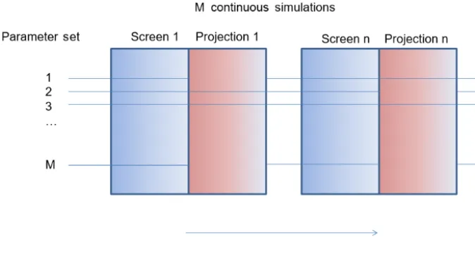
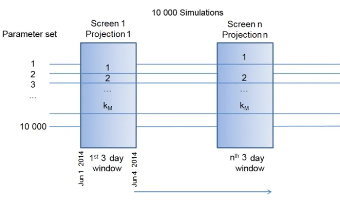
Figure 1.Schematic of the P-SET approach.Msimulations are run continuously from a model, of which the screen chooses a number from which to analyse a projection. The process is then repeated for subsequent screening periods, noting that theMsimulations run continuously through the previous projection periods even though they are not all selected for the previous projection period analysis.
DA is one way to improve hydrological predictions by merging models with observations, and DA methods can be categorized in a number of different ways (Liu and Gupta, 2007; Rakovec et al., 2015; Sun et al., 2016; Asch et al., 2016). One way of categorizing DA methods is by variational or sequential (statistical) methods. Variational approaches minimize the differences between observations and model output over a period of time, while sequential approaches as-similate observations as they are obtained. Another way of categorizing DA methods is by their time dependence. Usu-ally, smoothing problems attempt to make predictions for the past, filtering problems attempt to make predictions for the present, and forecasting problems attempt to make pre-dictions for the future. DA can include methods that help resolve problems related to estimating states, assessing pa-rameters and identifying the appropriate model structure (Liu and Gupta, 2007). Most applications of DA focus on merging state variables in a model with corresponding observations, while a few methods combine state and parameter estimation to improve predictions (e.g. Vrugt et al., 2005; Moradkhani et al., 2005a, b; Drécourt et al., 2006; Labarre et al., 2006; Qin et al., 2009; Nie et al., 2011; Xie and Zhang, 2013; Bi et al., 2014). However, none of these methods ensure that parameters and states are compatible with one another due to the statistical nature of parameter and state estimation ap-plied in the approaches.
In this paper, a new and very simple method that ensures parameter and state compatibility is presented for short-term hydrological ensemble prediction (up to 3 days). We call this approach parameter-state ensemble thinning (P-SET). The approach is described with the intention of making clear how to implement it with a wide variety of models in
data-rich or data-sparse watersheds, and examined here using a parameter-intensive, deterministic hydrologic land-surface scheme in a data-sparse watershed. The case studies include model structural and parameter errors, which are inevitable regardless of the model being used or the basin being mod-elled, to evaluate the ability of the P-SET approach.
The initial case studies are hindcasting exercises that reduce data and model structural uncertainty as much as possible, followed by a more realistic forecasting exam-ple (albeit in hindcasting mode) that incorporates data in-put uncertainty using Environment and Climate Change Canada’s (ECCC’s) meteorological Regional Ensemble Pre-diction System (REPS) to drive the model.
2 Methodology
2.1 The P-SET approach
are tied to one another (given the same initial conditions and model structure), both the parameters and states are drawn from the entireMsimulations for the projection period.
For a single screen-projection period, this approach is also described by Algorithm 1. This algorithm has similarities to approximate Bayesian computation (ABC, Biau et al., 2015). However, as described by Sadegh and Vrugt (2013), ABC can only be used with a stochastic operator. Sadegh and Vrugt (2013) use a deterministic equivalent of ABC to de-termine an initial distribution of suitable parameter values. The case study presented in this paper uses Latin hypercube sampling (LHS, McKay et al., 1979) to determine an initial distribution of parameter values. The P-SET approach, how-ever, reduces an initial set of parameter values (and their as-sociated state variables) for analysis during a prediction pe-riod. Each prediction period begins with the same initial en-semble, but the screening criteria are free to select a different sub-set of simulations for each separate prediction period. The interested reader is directed to the publications in paren-theses for applications of ABC and its deterministic equiva-lent in hydrology (Nott et al., 2012; Sadegh and Vrugt, 2013; Vrugt and Sadegh, 2013; Sadegh and Vrugt, 2014; Sadegh et al., 2015; Vrugt and Beven, 2018). The approach also has similarities to Bayesian recursive estimation (BaRE, Thie-mann et al., 2001) and the parameter identification method based on the localization of information (PIMLI, Vrugt et al., 2002). However, P-SET does not use any stochastic perturba-tion.
Algorithm 1Pseudo-code of the P-SET algorithm – adapted from Biau et al. (2015)
Require: A positive integerMand an integerkMbetween 1 andM.
fori=1 toMdo
generateyifrom the each member (θi) of the initial
ensemble of parameter sets. end for
returnTheθis such thats(yi)is among thekM-nearest neighbours ofs0.
In the context of the P-SET approach for hydrological pre-diction,θiis theith parameter set. In Biau et al. (2015), only
thekM-nearest neighbours between the statistic representing the observations, s0, and simulations, s(yi), for the
screen-ing period are kept for analysis. The case study presented below alters the selection criteria by using a distance func-tion (root mean squared error) to determine the discrepancy between the observations and the simulations, rather than in-dependent statistical properties (such as mean and standard deviation) of the two.
In the P-SET approach, we can disregard the notion of finding a distribution of parameter sets that fits the entire streamflow record of interest. Instead, we look for a collec-tion of plausible parameter sets, locate a certain number of these that generate the “best” results for the screening
pe-riod under consideration, and then evaluate how well these parameters and states perform for the projection period. The process is then repeated to find new parameter sets and states for consideration in successive projection periods. There are a number of ways in which screen and projection periods can be formulated. A number of such formulations are de-scribed in Sect. 2.7, which should clarify the generic process described in this paragraph. It is important to note that if the screen period is a hindcast, the projection period can be anal-ysed for its forecasting potential. Otherwise, the projection period can be analysed to help identify model structural er-rors.
2.2 Case study basin description
The study watershed is 1324 km2and is drained by the Lit-tle Pic River near Coldwell, Ontario, Canada, just north of Lake Superior (Fig. 2). The streamflow gauge (02BA003) is between the communities of Terrace Bay and Marathon and has been operated by the Water Survey of Canada from 1972 to the present. There are no precipitation measurements in the basin, but the surrounding region’s annual precipitation ranges from 654 to 879 mm, with the mean summer rainfall ranging from 231 to 298 mm (Crins et al., 2009). The mean annual temperature ranges from −1.7 to 2.1◦C (Mackey et al., 1996). The sub-surface sits on Precambrian Shield with significant amounts of volcanic rock, greenstone, silt-stone, and shale (Sutcliffe, 1991). The dominant land cover in the basin is mixed forest, followed by coniferous forest, water, sparse forest, and deciduous forest (Crins et al., 2009). The streamflow regime is characterized by frozen conditions through the winter months (November to April), but has been known to produce a spring freshet as early as March. Summer and autumn peaks can be on the same order of magnitude as the spring freshet, but are more often smaller. The peak flow is usually in May and the highest daily discharge recorded is 269 m3s−1on 30 June 2008.
2.3 The semi-distributed hydrologic land-surface scheme
The model used to simulate the streamflow is the MESH semi-distributed hydrological land-surface scheme (Pietron-iro et al., 2007), configured with the Canadian Land-Surface Scheme (CLASS, Verseghy, 1991; Verseghy et al., 1993), the hydrologic routing from WATFLOOD (Kouwen and Mousavi, 2002), and additional hydrological processes to better simulate surface and sub-surface lateral flow across the landscape to the river (Soulis et al., 2000, 2011).
classifica-Figure 2.Little Pic River basin near Coldwell, Ontario, Canada.(a)Location of the basin and legend,(b)basin outline with respect to ecodistrict,(c)river network and gauge location (02BA003), and(d)land cover (MW is mixed wood, CF is coniferous forest, BL is broadleaf forest, W is water, and O is other).
tion comes from the LCC2000-V product originating from classified Landsat 5 and Landsat 7 satellite images and the soils information comes from the ecodistricts classification of the national ecological framework for Canada (Agriculture and Agri-Food Canada, 2015). The basin fits within ecodis-trict 389 – Long Lake.
Table 1 shows the estimated percentages of each land cover present in the basin as defined by the LCC2000-V product. Based on this classification, the two dominant land covers are coniferous and broadleaf forest, which are often mixed. Without knowing more specific information about the land cover, the mixed forests are assumed to be 50 % conif-erous and 50 % broadleaf, resulting in an estimate of 48 % coniferous and 39 % broadleaf. These values are then arbi-trarily rounded up to 50 % coniferous and 40 % broadleaf in the model representation of land cover. The remaining 10 % of land cover inevitably includes parametric uncertainty due to the model’s inability to properly represent the 8 % of the basin that is covered by small lakes.
[image:4.612.100.498.65.348.2]Figure 2 illustrates (a) the location of the basin, (b) ecodis-trict boundary and model grid, (c) river network and gauge location, and (d) land cover. Sub-grid variability of each grid is handled via the CLASS tile with each grid being repre-sented by the same ecodistrict.
Table 1.Land-cover percentages based on the LCC2000-V Landsat product.
Land cover Percentage
Water 8
Coniferous dense forest 23 Broadleaf dense forest 13
Mixed wood 53
Other 3
2.4 Forcing data
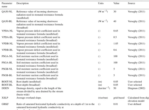
[image:4.612.352.503.445.523.2]Precipita-Table 2.Fixed land-cover parameters.
Parameter Description Units Value Source
name
QA50-NL Reference value of incoming shortwave (W m−2) 30 Verseghy (2011)
radiation used in stomatal resistance formula (needleleaf)
QA50-BL Reference value of incoming shortwave (W m−2) 40 Verseghy (2011)
radiation used in stomatal resistance formula (broadleaf)
VPDA-NL Vapour pressure deficit coefficient used in ( ) 0.65 Verseghy (2011)
stomatal resistance formula (needleleaf)
VPDA-BL Vapour pressure deficit coefficient used in ( ) 0.5 Verseghy (2011)
stomatal resistance formula (broadleaf)
VPDB-NL Vapour pressure deficit coefficient used in ( ) 1.05 Verseghy (2011)
stomatal resistance formula (needleleaf)
VPDB-BL Vapour pressure deficit coefficient used in ( ) 0.6 Verseghy (2011)
stomatal resistance formula (broadleaf)
PSGA-NL Soil moisture suction coefficient used in ( ) 100 Verseghy (2011)
stomatal resistance formula (needleleaf)
PSGA-BL Soil moisture suction coefficient used in ( ) 100 Verseghy (2011)
stomatal resistance formula (broadleaf)
PSGB-NL Soil moisture suction coefficient used in ( ) 5 Verseghy (2011)
stomatal resistance formula (needleleaf)
PSGB-BL Soil moisture suction coefficient used in ( ) 5 Verseghy (2011)
stomatal resistance formula (broadleaf)
ROOT-NL Root depth (needleleaf) (m) 0.05 User selected
ROOT-BL Root depth (broadleaf) (m) 0.05 User selected
DDEN Drainage density, equal to the length of the (km km−2) 50 Dingman (2002)
stream divided by area drained by the stream (basin wide)
XSLP Average overland slope. (rise/run) grid-based Calculated from digital
elevation model GRKF Ratio of saturated horizontal hydraulic conductivity at a depth of 1 m to the ( ) 0.01 User defined
saturated horizontal hydraulic conductivity at the surface (basin wide)
( ): dimensionless.
tion Analysis (CaPA, Mahfouf et al., 2007; Lespinas et al., 2015), which is an assimilation of ground-based observations and GEM precipitation forecasts. For the third case study in-cluding forcing input data uncertainty, an ensemble of me-teorological inputs is obtained from ECCC’s Meme-teorological Regional Ensemble Prediction System (REPS). The REPS provides 72 h forecasts twice daily.
2.5 Parameter selection
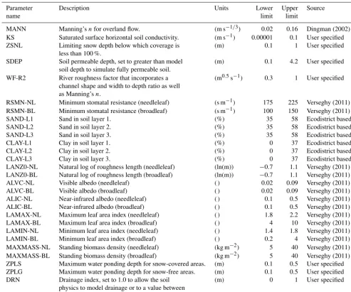
H-LSSs contain many parameters and there is a large body of scientific literature examining various techniques for effec-tively estimating parameters (for a brief review, see Matott et al., 2009). The method that was used in this study is Latin hypercube sampling (LHS, McKay et al., 1979). Twenty-eight parameters were perturbed based on the results of a simple study (not shown) comparing the perturbation of 6, 15, and 28 parameters. Table 2 shows the parameter values that were fixed during the simulations, while Table 3 shows the ranges for parameters that were perturbed. The
parame-ters that were perturbed were based on the lead author’s ex-perience with the model. Parameter intervals were set based on the ranges found in sources identified under the source column of Table 3. In the case of user-specified parameters, these were set by the lead author.
[image:5.612.51.543.85.448.2]Table 3.Ranges for the perturbed parameters.
Parameter Description Units Lower Upper Source
name limit limit
MANN Manning’snfor overland flow. (m s−1/3) 0.02 0.16 Dingman (2002) KS Saturated surface horizontal soil conductivity. (m s−1) 0.00001 0.1 User specified ZSNL Limiting snow depth below which coverage is (m) 0.1 1 User specified
less than 100 %.
SDEP Soil permeable depth, set to greater than model (m) 0.1 4.2 User specified soil depth to simulate fully permeable soil.
WF-R2 River roughness factor that incorporates a (m0.5s−1) 0.3 1 User specified channel shape and width to depth ratio as well
as Manning’sn.
RSMN-NL Minimum stomatal resistance (needleleaf) (s m−1) 175 225 Verseghy (2011) RSMN-BL Minimum stomatal resistance (broadleaf) (s m−1) 100 150 Verseghy (2011)
SAND-L1 Sand in soil layer 1. (%) 35 58 Ecodistrict based
SAND-L2 Sand in soil layer 2. (%) 35 58 Ecodistrict based
SAND-L3 Sand in soil layer 3. (%) 35 58 Ecodistrict based
CLAY-L1 Clay in soil layer 1. (%) 0 37 Ecodistrict based
CLAY-L2 Clay in soil layer 2. (%) 0 37 Ecodistrict based
CLAY-L3 Clay in soil layer 3. (%) 0 37 Ecodistrict based
LANZ0-NL Natural log of roughness length (needleleaf) (ln(m)) −0.7 1.1 Verseghy (2011) LANZ0-BL Natural log of roughness length (broadleaf) (ln(m)) −0.7 1.1 Verseghy (2011) ALVC-NL Visible albedo (needleleaf) ( ) 0.02 0.09 Verseghy (2011)
ALVC-BL Visible albedo (broadleaf) ( ) 0.02 0.09 Verseghy (2011)
ALIC-NL Near-infrared albedo (needleleaf) ( ) 0.1 0.5 Verseghy (2011) ALIC-BL Near-infrared albedo (broadleaf) ( ) 0.1 0.5 Verseghy (2011) LAMAX-NL Maximum leaf area index (needleleaf) ( ) 1.8 2.2 Verseghy (2011) LAMAX-BL Maximum leaf area index (broadleaf) ( ) 4 10 Verseghy (2011) LAMIN-NL Minimum leaf area index (needleleaf) ( ) 1.4 1.8 Verseghy (2011) LAMIN-BL Minimum leaf area index (broadleaf) ( ) 0.2 4 Verseghy (2011) MAXMASS-NL Standing biomass density (needleleaf) (kg m−2) 5 40 Verseghy (2011) MAXMASS-BL Standing biomass density (broadleaf) (kg m−2) 5 40 Verseghy (2011) ZPLS Maximum water ponding depth for snow-covered areas. (m) 0.1 0.5 User specified ZPLG Maximum water ponding depth for snow-free areas. (m) 0.1 0.5 User specified DRN Drainage index, set to 1.0 to allow the soil (m) 0 1 User specified
physics to model drainage or to a value between 0.0 and 1.0 to impede drainage.
2.6 Projection periods for short-term hydrological prediction
This paper is focused on short-term hydrological ensem-ble prediction (up to 3 days), with an interest in using the ECCC meteorological REPS to force a more comprehen-sive Hydrological-Ensemble Prediction System (H-EPS). As such, projection periods are defined as the 3-day windows of time from the beginning of each ECCC-REPS run at 00:00 and 12:00 UTC. The red and pink bars in Fig. 3 illus-trate 12 projection periods beginning on 00:00 UTC, 20 July to 12:00 UTC, 25 July 2014. The remainder of Fig. 3 is de-scribed in Sect. 2.7.2.
2.7 Ensemble selection methodologies
The total population of model runs is generated by settingM to 10 000 in Algorithm 1 and using LHS to generate the 10 000 parameter sets from a uniform prior distribution of 28 parameters based on the ranges shown in Table 3. MESH is run with each of the 10 000 parameter sets in a continuous simulation mode to generate streamflow values (y) for the period of June 2002 to November 2014.
The “thinning” is performed by screening the total popu-lation of 10 000 model runs to generate an ensemble of the “best” model runs to be used in the subsequent projection pe-riod. Algorithm 2 represents the specific implementation of Algorithm 1 used in this paper.
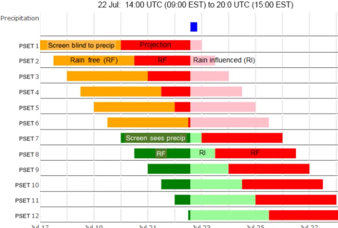
Figure 3.Preceding streamflow screen and projection periods for 17 to 28 July 2014 using hourly streamflow. This figure is fully explained in Sect. 2.7.2 and 2.8.2.
Algorithm 2 Pseudo-code of the P-SET algorithm imple-mentation in this paper
Require: A positive integer 10 000 (M) and an integer (kM) between 1 andM(in this study, a sensitivity analysis ofkMis
performed by settingkM=5, 10, 20, 30, 40, and 50). fori=1 to 10 000do
generate streamflowi(yi) using the model (MESH)
end for
returnThe parameter sets with the lowestkMRMSE values between observed and simulated streamflow values from the
10 000 model runs for the screening period.
1. optimal hindcast of 3-day projections; 2. preceding streamflow screen;
3. hindsight parameter constraint and preceding 3-day streamflow screen;
4. H-EPS.
An initial evaluation of the P-SET screens requires some sources of uncertainty to be minimized. In particular, stream-flow observations and precipitation uncertainty are consid-ered, and questions around the model’s ability to manage snow processes are simply avoided.
The quality of a streamflow observation is commonly known to be affected by ice, the occurrence of which is noted in the Water Survey of Canada database of stream-flow. For the Little Pic River watershed, ice on the river can occur as early as November and as late as April. In addi-tion, prior to the spring freshet, the streamflow contains
al-most no information that could assist in predicting future streamflow. The future flow primarily depends on other land-surface characteristics such as snow water equivalent and frozen ground. Because the immediate interest is in evaluat-ing the P-SET screens when snow or ice on the ground is not present, the analysis is only performed from 1 June to 31 Oc-tober for 2014, with some qualitative analysis beginning on 1 May 2014.
Each of the four P-SET configurations is described below. 2.7.1 Optimal hindcast of 3-day projections
Since there are no precipitation observations in the basin, but there are some precipitation gauges nearby which are used in the generation of CaPA, the approach is initially tested with reduced precipitation uncertainty by forcing the model with CaPA.
Figure 4.Schematic of P-SET for the optimal hindcast of 3-day projections used in this study; 10 000 simulations are run continuously through the MESH model, of which the screen chooses a number (kM) for the hindcast analysis. The process is then repeated for subsequent screening periods.
Figure 5.Schematic of P-SET for the preceding streamflow screen; 10 000 simulations are run continuously through the MESH model, of which the screen chooses a number (kM) from which to analyse a projection. The process is then repeated for subsequent screening periods, noting that theMsimulations run continuously through the previous projection periods even though they are not all selected for the previous projection period analysis.
2.7.2 Preceding streamflow screen
Figure 5 illustrates the preceding streamflow screen. In this study, 10 000 simulations are run continuously through the MESH model, of which the screen chooses a number (kM) from which to analyse for a projection period. The process is
then repeated for subsequent screening periods, noting that the M simulations run continuously through the previous projection periods even though they are not all selected for the previous projection period analysis.
screen considered for a 3-day screening period (other screen-ing period lengths are examined in the results). In this figure, 12 screen periods are shown in orange and green for 17 to 25 July 2014. The first screen period is represented by the orange bar near the top of the figure beside the PSET1 la-bel. This screen period runs from 00:00 UTC on 17 July to 00:00 UTC on 20 July 2014. During this 3-day period, the “best” parameter sets are selected based on how the model simulates the observed streamflow. The simulations for these top performing parameter sets are then extended for 3 more days, which is considered to be the projection period.
This process is then repeated 12 h later. The second screen-ing period is represented by the orange bar illustrated just be-low the first screening period and labelled PSET2 in the fig-ure. This screening period runs from 12:00 UTC on 17 July to 12:00 UTC on 20 July 2014. During this 3-day period, the “best” parameter sets are selected based on how the model simulates the observed streamflow. Although there is consid-erable overlap between the first and second screening peri-ods, the second screening period begins and ends 12 h af-ter the first screening period, producing a new ensemble of “best” parameter sets. The simulations for these new param-eter sets are then extended for 3 days, which is considered to be a new projection period that also begins and ends 12 h after the previous projection period.
The process is then continually repeated every 12 h as shown by the remainder of the bars shown in the rows la-belled PSET3 to PSET12. Each instance of the screen and projection periods represents a single application of P-SET, which is why each row is labelled as such. We call this ap-proach the preceding streamflow screen because the projec-tion periods shown in red and pink occur immediately after the screening periods.
One important consideration that becomes relevant in the analysis is the 6 h of precipitation that occurred on 22 July from 14:00 to 20:00 UTC. This is illustrated by the small blue bar at the top and near the middle of Fig. 3. Some of the projection periods “see” this precipitation event (illus-trated by the green bars) and some do not (illus(illus-trated by the orange bars). As will be explained more fully in Sect. 2.8.2, the analysis is split according to the sub-periods of the screen and projection periods that (a) occur during and just after the precipitation event (the light green and pink bars), and that (b) occur when it is otherwise rain-free (orange, dark green, and red bars).
To properly examine the effectiveness of the P-SET ap-proach, a sensitivity analysis is performed for the length of the screen period as well as forkM in Algorithms 1 and 2.
The length of the screen period is tested for 3, 10, 20, 30, and 40 days, whilekM is tested for values of 5, 10, 20, 30,
40, and 50.
2.7.3 Hindsight parameter constraint and preceding 3-day streamflow screen
The third ensemble considered is very similar to the pre-ceding streamflow screen with a screening period of 3 days. However, to constrain the parameter space further than de-termined by LHS, the population of parameter sets is re-duced by selecting a sub-set from the initial population of 10 000 parameter sets. The sub-set is selected by confining the parameter values based on model simulations that re-spond well during precipitation events in 2014. Figure 6 il-lustrates this screen and more details are provided in Sect. 3.3 of the results. This ensemble represents an approach that can-not be used in a forecasting context, but does represent a proxy for other parameter-constraining methods that are ex-plored in the discussion and helps to examine model struc-tural errors.
2.7.4 H-EPS
Of course it is not often known for sure whether precipitation will occur in the future, and certainly not the amount of pre-cipitation that will occur. As a result, ECCC’s Meteorolog-ical REPS is also used with the 1 June to 31 October 2014 data in a hindcasting mode to examine how the P-SET ap-proach can be used in a true forecasting context. At 00:00 and 12:00 UTC every 12 h from 1 May to 31 October 2014, the top 10 parameter-state pairs from the screen period and dif-ferent projection periods are run for 3 days using the forc-ing data from the 20 members of the REPS, for a total of 200 H-EPS members. This analysis is performed for a hind-sight parameter constraint and preceding 3-day streamflow screen and akMvalue of 10 for illustrative purposes.
The only other use of ECCC’s REPS as a part of a H-EPS is found in Abaza et al. (2013), in which the Cana-dian operational meteorological Global Ensemble Prediction System (GEPS) was compared with the REPS and the deter-ministic 15 km GEM NWP forcing of the province of Que-bec’s operational streamflow forecasting system. The study found that both the GEPS and REPS outperformed a deter-ministic run for eight watersheds ranging in size from 355 to 5820 km2. The REPS was also found to be superior to the GEPS in terms of its ability to predict forecast uncertainty.
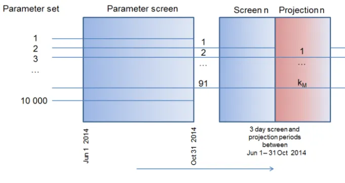
Figure 6.Schematic of P-SET for the hindsight parameter constraint and preceding 3-day streamflow screen used in this study. 10 000 sim-ulations are run continuously through the MESH model. The original 10 000 parameter sets are reduced to 91 parameter sets based on a hindsight analysis of parameters that are shown to be important during precipitation events between 1 June and 31 October 2014. These remaining 91 parameter sets are then selected for analysis in the preceding streamflow screen as ifM=91 in Algorithm 1.
2.8 Verification
Demargne et al. (2010) differentiate diagnostic verification for evaluating the performance of a system from real-time verification for helping end-users make decisions about the future. The verification performed here is done for the first of these objectives: evaluating the performance of a system.
2.8.1 Verification of the ensemble selection methodologies
First, a qualitative analysis is undertaken to take advantage of the human brain’s ability to synthesize information. The results are then quantitatively verified using the Ensemble Verification System (EVS, Brown et al., 2010). To exam-ine the quality of the ensemble mean when compared with the corresponding observation, the mean error (ME) is culated. Then the quality of the ensemble distribution is cal-culated using rank histograms. Finally, the skill relative to us-ing the current streamflow as the forecast is calculated usus-ing the mean continuous ranked probability skill score (CRPSS). The reference forecast in this study is taken to be the mea-sured streamflow at 00:00 and 12:00 UTC each day as the forecast for the next 72 h. This reference forecast is a per-sistence forecast, which assumes the streamflow is persistent for the forecast period.
The ME measures the average difference between a set of forecasts and corresponding observations. In this case, it measures the average difference between the mean average
of the ensemble forecast (Y) and the observation (x) as fol-lows:
ME= 1 n
n
X
i=1
Yi−xi. (1)
The ME may be positive, zero, or negative. A positive value represents an ensemble mean that is positively biased while a negative error represents an ensemble mean that is negatively biased. A value of zero represents an absence of bias in the ensemble mean.
The rank histogram measures the reliability of an en-semble forecasting system. It involves counting the fraction of observations that fall between any two ranked ensemble members in the forecast distribution. For an ensemble fore-cast containing mensemble members ranked in ascending order, there arem−1 spaces between any two ranked en-semble members and two spaces at the ends (above and be-low the ensemble forecast range) for a total ofm+1 spaces (s1, . . . ,sm+1). The corresponding observationhfor each en-semble forecast will fall within one of the spaces.
hi=
1 n
n
X
j=1
1xj∈sij , (2)
wherehi is the fraction in theith bin,xj is thejth observed
value,sij is theith gap associated with thejth forecast, and
1{·}is a step function that gives a value of 1 if the condition is met and 0 otherwise.
sys-tem in terms of the mean continuous ranked probability score (CRPS). The CRPS measures the average square error of a probability forecast across all possible event thresholds. The CRPSS comprises a ratio of the CRPS for the forecast-ing system to be evaluated, CRPSEVAL, and the CRPS for a reference forecasting system, CRPSREF.
CRPSS=CRPSREF−CRPSEVAL CRPSREF
(3) As a measure of the average square error in probability, val-ues for the CRPS approaching zero are better. As a result, values for the CRPSS closer to one are better as this illus-trates that CRPSEVAL<CRPSREF.
2.8.2 Splitting the analysis based on rainfall
The qualitative analysis shown in the following Results sec-tion illustrates that there is a significant difference in the abilities of the P-SET configurations to effectively project streamflow when it is raining and when it is not raining. As a result, the quantitative analysis is split into two parts: (1) for periods in which it is raining and just afterwards (for the re-mainder of each respective screen or projection period), and (2) for periods in which it is otherwise not raining.
Note that these periods do not necessarily correspond to the rising-limb and recession periods of the hydrograph since the river does not always respond strongly to the precipitation for the time period of study in this basin. As a result, for lack of better terminology, these periods are hereafter referred to as “rain-influenced” and “rain-free”. It would be more cor-rect to say “periods during and immediately after the rainfall within the 3-day period” and “otherwise rain-free”, but this terminology would be cumbersome throughout the remain-der of the paper. Furthermore, it is also important to note that the terms “rain-influenced” and “rain-free” only refer to a time period rather than the discharge of the river. The time periods that these terms refer to are the stretch of time under consideration in the analysis.
Recall the description for Fig. 3 in Sect. 2.7.2. for il-lustrating the difference between “rainfall” and “rain-free”. The screen periods are rain-free for the 22 July rain event in PSET1 through to PSET12 as shown by the orange and dark green bars, while the screen periods are rain-influenced in PSET7 through to PSET12 as shown in the light green bars. Similarly, the projection periods are rain-influenced in PSET1 to PSET6 as shown by the pink bars and rain-free in PSET1 to PSET12 as shown in the red bars. In both cases (screen and projection), the rain-influenced period is con-sidered to be from the beginning of the rainfall (22 July, 09:00 EST in Fig. 3) to the end of the corresponding screen or projection period that “sees” the precipitation.
Recall that MESH is run in a continuous simulation mode for the period of June 2002 to November 2014, with a de-tailed analysis of the ensemble selection methodologies from 1 June to 31 October 2014. Within this time period, there are
five significant precipitation events. The beginning and end-ing of the precipitation events are considered as follows:
– 22 July, 14:00 UTC (09:00 EST) to 20:00 UTC (15:00 EST);
– 11 August, 14:00 UTC (09:00 EST) to 20:00 UTC (15:00 EST);
– 10 September, 08:00 UTC (03:00 EST) to 11 Septem-ber, 02:00 UTC (10 SeptemSeptem-ber, 21:00 EST);
– 19 September, 20:00 UTC (15:00 EST) to 20 Septem-ber, 20:00 UTC (15:00 EST);
– 3 October, 08:00 UTC (03:00 EST) to 20:00 UTC (15:00 EST).
For the rain-influenced and rain-free periods, the quality of the ensemble mean, distribution and skill are compared. The 3 June rain-influenced period is not assessed due to the fact that it was not a projection period in the preceding stream-flow screen.
2.8.3 Verification of the H-EPS
As with the earlier analysis when precipitation uncertainty is minimized, the mean error and CRPSS are calculated for streamflow for both rain-influenced and rain-free periods as determined by precipitation events in the basin. The overall mean error and CRPSS are also calculated.
The mean error, rank histograms, and CRPS of the REPS precipitation ensemble mean are calculated using CaPA as the observation. The CRPSS is also calculated using the June to October CaPA “climatology” as the reference fore-cast. The mean error, CRPS, and CRPSS are calculated above and below the 90th percentile of CaPA precipitation (0.42 mm h−1).
3 Results
The results are ordered according to the ensemble selection methodologies. In all cases, the projection time period of in-terest is short-term, which is defined here as 3 days.
3.1 Optimal hindcast of 3-day projections
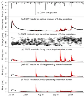
Figure 7.CaPA precipitation(a)for all simulations shown in this figure.(b)Observed streamflow (black) and top 10 streamflow values (red) for the optimal hindcast of 3-day projections.(c)Corresponding basin-wide storage values for the optimal hindcast of 3-day projections. (d)Top 10 preceding streamflow projections for each of the 3-day screen periods.(e)Top 10 preceding streamflow projections for each of the 10-day screen periods.(f)Top 10 preceding streamflow projections for each of the 20-day screen periods. The black lines in(d–f)show observed streamflow with differenty-axis scaling than in(b).
each of the parameter-state pairs chosen by the optimal hind-casts. These storage results will be discussed later.
For this study, the qualitative results in Fig. 7b illustrate that CaPA precipitation cascades to reasonable streamflow values for the time period examined. A quantitative analy-sis compares these results to the other ensemble selection methodologies, but a qualitative analysis is first performed for each of the remaining approaches.
3.2 Preceding streamflow screen
One manner in which to screen the parameter sets (and as-sociated states) is to consider only the preceding streamflow. In this study, the best RMSE values from the preceding days of streamflow are used to determine the parameter sets to use for the prediction of the subsequent 3 days of streamflow. This process is repeated twice daily at 00:00 and 12:00 UTC (19:00 and 05:00 LT – local time – for the basin in question) for 1 June to 31 October 2014.
Figure 8.A single screen-projection period for two neighbouring time periods. For the two sub-plots in(a)the projection begins at 07:00 LT (local time), 22 July 2014 (12:00 UTC). For the two sub-plots in(b)the projection begins at 19:00 LT, 22 July 2014 (00:00 UTC, 23 July). The upper plot of each sub-figure shows CaPA precipitation and instantaneous storage. The lower plot shows observed streamflow (black), the top 10 runs for the screening period (blue), and the corresponding streamflow projections (red).
3.3 Hindsight parameter constraint and preceding 3-day streamflow screen
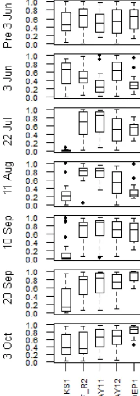
The third screen explored here is one in which the top sim-ulations are selected based on the preceding streamflow and parameter ranges that are proven to be important during the 2014 precipitation events. Figure 9 shows parameters that are particularly sensitive during six precipitation events. Each parameter is normalized between 0 and 1. Based on a sub-jective visual analysis of these box-plots, the 10 000 pa-rameter sets are reduced to 91 papa-rameter sets by confin-ing the values of the normalized parameters as follows: KS1<0.1, WF_R2>0.6, CLAY11>0.5, CLAY12>0.5, SDEP1>0.2. Using the preceding streamflow screen with these 91 parameter sets to obtain the top 10 runs for each 3-day period yields Fig. 10. This approach of identifying parameter ranges based on periods of hydrological signifi-cance is similar to the DYNIA approach described by Wa-gener et al. (2003), albeit much less rigorous. With the ex-ception of the 3 June precipitation event, these results are
clearly much better than those found in the unconstrained 3-day screen shown in Fig. 7c. Although this method clearly cannot be used in a forecasting context, the significance of these findings is examined in the discussion.
3.4 A quantitative comparison of screens
con-Figure 9.Importance of (normalized) parameters that see precipita-tion. The top set of box-plots shows that none of the top parameter sets have identifiable parameter values prior to the 3 June 2014 pre-cipitation event. This result is similar to all parameter sets imme-diately prior to precipitation events that do not see the events. The remaining sets of box-plots show the parameter ranges for the top simulations during precipitation events.
strained parameters performs close to the optimal hindcast with only a slight over-prediction of the observed flows.
The number of “top” runs selected (kM) does not appear to have much influence over these mean error results. As a consequence the remainder of the analysis is performed with a value ofkM=10.
Using the current streamflow as the reference forecast. Ta-ble 5 shows the skill of the optimal hindcast, 20-day screen and 3-day screen with constrained parameters. The opti-mal hindcast exhibits a relatively high skill for rain-free and rain-influenced periods. For the rain-free periods, the 20-day
screen shows some skill for the 48 and 72 h forecast, while the 3-day screen with constrained parameters shows no skill. For the rain-influenced periods, the only screen that shows any skill is the 3-day projection with constrained parame-ters. These results quantify the qualitative analysis shown in Figs. 7 and 10.
3.5 H-EPS
To address the question of how this data assimilation ap-proach could be used in a forecasting context, a full H-EPS is used to force selected parameter-state ensemble members with ECCC’s Meteorological Regional Ensemble Prediction System (REPS), as described in the methodology section. Two sets of parameter-state ensembles are selected to see how the REPS performs. The ensembles are based on (1) the optimal hindcast of 3-day projections and (2) the hindsight parameter constraint and preceding 3-day streamflow screen. These ensembles were selected because they were the only methods that showed any skill in the rain-influenced periods. Of course, neither of these ensembles can be used in oper-ational forecasting, so they are used as a proxy for illustra-tive purposes assuming that the limitations of the preceding streamflow screen can be addressed as explored in the dis-cussion. Although these two ensembles are “unforecastable”, performing this analysis provides a more meaningful mech-anism to examine model structural and forcing errors.
Figure 11a shows CaPA (reddish brown) and the 20 REPS precipitation members (blue). The resulting 200 streamflow ensembles (recall thatkM=10) are shown in Fig. 11b, with the black line representing the observed streamflow, the or-ange lines coming from the hindsight-constrained parameter and preceding 3-day streamflow screen, and the green lines coming from the optimized hindcast. Even for the optimal hindcast, which shows near-perfect alignment with the ob-served streamflow when forced with GEM and CaPA, the REPS members that overestimate the precipitation have an impact on the resulting ensemble of streamflows.
[image:14.612.96.239.69.473.2]Table 4.Mean error (m3s−1) as an assessment of the ensemble mean streamflow for the reference forecast, the optimal hindcast, and various configurations of P-SEDA. The value ofkMfrom Algorithms 1 and 2 varies from 5 to 50 as shown. Rain-influenced and rain-free periods from June to October 2014 as described in the text.
Rain-free Rain-influenced
kM kM
5 10 20 30 40 50 5 10 20 30 40 50
Reference forecast 2 2 2 2 2 2 −8 −8 −8 −8 −8 −8
Optimal hindcast 0 0 0 0 0 0 3 3 3 4 4 4
3-day screen 1 2 2 2 2 2 41 42 45 46 46 46
10-day screen 1 1 2 2 2 2 11 10 12 12 12 13
20-day screen 1 1 1 2 2 2 4 5 7 8 9 9
30-day screen 2 1 2 2 3 3 4 6 8 9 9 9
40-day screen 2 2 3 3 3 4 6 7 8 9 9 9
[image:15.612.154.443.418.581.2]3-day screen with constrained parameters 3 4 4 4 5 5 2 4 4 5 5 6
Figure 10.Projection period results after screening based on parameter values and preceding streamflow.
Figure 11.Results of the H-EPS for the 3-day period beginning at 06:00 EST (Eastern Standard Time) on 21 July 2014. The reddish brown line in(a)is the Canadian Precipitation Analysis (CaPA), while the blue lines represent the 20 Regional Ensemble Prediction System (REPS) precipitation traces. The single black line in(b)is the observed streamflow. The orange and green lines show the 200 H-EPS streamflow traces for the projection periods of the constrained parameter with a preceding 3-day streamflow screen, and the optimized hindcast.
precipitation overestimates the CaPA precipitation. In the top 10 % of CaPA precipitation values, however, the REPS mean underestimates the CaPA precipitation. The rank histograms (not shown) indicate that the ensemble members tend to underestimate precipitation, although some REPS members
Table 5.Mean CRPSS as an assessment of the ensemble skill from P-SEDA for rain-influenced and rain-free periods from June to Octo-ber 2014. The configurations considered here are the optimal hindcast, the 3-day projection for the 20-day screen, and the 3-day projection for the 3-day screen with constrained parameters. The reference forecast is the measured streamflow at 00:00 and 12:00 UTC each day as the forecast for the next 72 h. The value ofkm=10 from Algorithms 1 and 2 in all cases.
Rain-free Rain-influenced Forecast hour Forecast hour
24 48 72 24 48 72
Optimal hindcast 0.85 0.92 0.90 0.76 0.83 0.70
20-day screen −0.09 0.27 0.42 −0.37 −0.15 −0.08 3-day screen with constrained parameters −0.74 −0.22 −0.02 0.41 0.45 0.42
4 Discussion
The discussion is organized around three questions. The first question looks at whether or not the P-SET approach is capa-ble of reproducing observed streamflow, which corresponds to the optimized hindcast. The second question considers the effectiveness of the remaining screening approaches. The third question revolves around the more realistic example of using the approach in a full H-EPS. Finally, advantages and limitations of the approach are discussed.
4.1 Given maximum data certainty, can the P-SET approach reproduce observed streamflow?
Although the P-SET approach could be applied to a hy-drological model with few parameters, the Canadian MESH model is used with many parameters perturbed, which in-creases the dimensionality of the problem. Although much simpler models tend to dominate the operational hydrologi-cal modelling community, part of the motivation behind us-ing a hydrologically enhanced land-surface scheme in the case study is to begin laying some foundation for using such parameter-intensive models for operational ensemble hydro-logical forecasting.
One major limitation to the way in which MESH is applied in this study is the use of the relatively inefficient Latin hy-percube sampling to determine the prior distribution of pa-rameter sets to be used with the P-SET approach. Despite this limitation, however, the results clearly show that the ap-proach can, with confidence in the precipitation forcing and streamflow, find parameter-state sets that match the observed hydrograph over successive periods of a few days. One pos-sible way of dealing with the uncertainty in precipitation is to perturb the CaPA precipitation field, as is examined by Car-rera et al. (2015).
The widely varying nature of the simulated basin storage for the selected runs for each 3-day period also highlights a limitation with the study. This limitation is in only using streamflow as the state variable to determine the top param-eters each time. Consider the following water balance equa-tion for the basin:P−E=R+dS/dt, whereP is precip-itation, E is evapotranspiration, R is runoff, and dS/dt is
the change in basin storage over time. Over the short time periods of a few days in short-term hydrological prediction, Ecan generally be ignored, leaving onlyP =R+dS/dt. In the hindcasting exercise presented in this part of the study, P andRare considered to be known and the only remaining term is dS/dt. So why does the analysis show such a wide range of basin storage terms for the best matching assimi-lated streamflow? The answer lies in the fact that it is not the basin storage that balances the equation, but rather the change in storage over the time period of interest. The model is capable of releasing or storing the appropriate amount of water in both rain-influenced and rain-free scenarios, and the model determines dS/dt based on the interaction of existing storage, model physics, and parameters.
The issue of widely varying simulated basin storage (Fig. 7c) also highlights the issue of equifinality, which is de-fined here as the idea that many different model simulations can produce acceptable results (Beven, 1993). The model is able to find many parameter-state sets that fit the streamflow for short periods of time. If only streamflow observations are available, the selected simulations are equifinal. How-ever, including the state of basin storage clearly shows that the parameter-state sets are not equal. If soil moisture obser-vations are also available and used, then the selected sim-ulations could be further constrained. Of course, including soil moisture observations to further constrain the selection of simulations would not remove equifinality. It would sim-ply make it more likely that the model is more accurately predicting both streamflow and soil moisture.
fur-Table 6.Mean error (mean H-EPS streamflow – observed) (m3s−1) as an assessment of the ensemble mean streamflow from the H-EPS (200 members) for rain-influenced, rain-free, and overall periods from June to October 2014.
Rain-free Rain-influenced Overall Forecast hour Forecast hour Forecast hour
24 48 72 24 48 72 24 48 72
Optimized hindcast 1 2 3 1 2 7 1 2 3
[image:17.612.107.488.99.169.2]3-day screen with constrained parameters 2 3 3 1 2 4 2 3 3
Table 7.Mean CRPSS as an assessment of the ensemble skill from the H-EPS for rain-influenced, rain-free, and overall periods from June to October 2014. The reference low-skill forecast is the measured streamflow at 00:00 and 12:00 UTC each day as the forecast for the next 72 h.
Rain-free Rain-influenced Overall
Forecast hour Forecast hour Forecast hour
24 48 72 24 48 72 24 48 72
Optimized hindcast 0.77 0.76 0.67 −0.33 0.12 0.01 0.71 0.70 0.60 3-day screen with constrained parameters −0.77 −0.31 −0.14 −1.2 −0.15 0.11 −0.80 −0.29 −0.11
ther constraints to give the results a more solid foundation. One of these constraints could be multi-objective calibration, or else further “thinning”, based on some aspects of storage in the model. One such possibility would be to examine the usefulness of the soil moisture and ocean salinity (SMOS) satellite (Mecklenburg et al., 2012; Jackson et al., 2012; Ri-dler et al., 2014).
Related to model structural error, the unresponsive stream-flow in this study is likely due to “fill-and-spill” dynamics (Spence, 2010). Being on the Precambrian Shield, and the starting point of many streams in the basin being small lakes, there are many parts of the basin that need to be filled-up before they contribute to streamflow. This physical process, especially with respect to the headwater lakes, is not rep-resented in the version of MESH used in this study. Future work should focus on this aspect more closely.
4.2 How well do different P-SET configurations work?
The issues of parameter time invariance and the most appro-priate model structures are generally secondary considera-tions in forecasting. The focus shifts from the exercise of im-proving the model and its parameterization to the exercise of making a more accurate prediction. The results presented from the various configurations tested, however, indicate that some thought is required to determine the appropriate param-eter sets at the appropriate times.
The only configurations in this study that show any skill in predicting streamflow when it rains are (a) the optimal hindcast of 3-day projections, and (b) the hindsight param-eter constraint and preceding 3-day streamflow screen. The manner in which the second of these approaches is applied in this study reveals that 91 of the original 10 000 LHS
pa-rameter sets can be used effectively with the P-SET approach to perform short-term predictions in the basin for the months of July to October 2014. The reduction of 10 000 parameter sets to 91 parameter sets is notable.
The fact that constraining the parameter sets allows for the approach to produce reasonable results throughout the pe-riod provides some assurance that the method has the pos-sibility of being able to predict streamflow with some skill in a forecasting context. The key, at least in part, is expected to be in using a method other than LHS to determine the ini-tial ensemble of parameter sets. Alternative approaches could use algorithms such as dynamically dimensioned search– approximation of uncertainty (DDS–AU) which have been shown to be more efficient than GLUE (Tolson and Shoe-maker, 2008). The prior can also be obtained by looking for parameter sets that perform well for different hydrolog-ical signatures (e.g. Zhang et al., 2014; Shafii and Tolson, 2015) or different hydrological scenarios which might in-clude streamflow responses to snowmelt, runoff over frozen ground, rain during wet conditions, rain during dry condi-tions, or whatever else can be considered a relevant hydro-logical event affecting streamflow.
[image:17.612.49.546.230.299.2]fore-Table 8.Mean error (mean REPS precipitation – CaPA), CRPS, and CRPSS (with JJASO 2014 “climatology” as reference forecast) for 1 June to 31 October 2014.
Threshold Mean error CRPS CRPSS
Forecast hour Forecast hour Forecast hour
24 48 72 24 48 72 24 48 72
Pr≤0.9 (0.42 mm h−1) 0.05 0.06 0.09 0.03 0.03 0.04 0.30 0.19 0.08 Pr>0.9 (0.42 mm h−1) −0.14 −0.21 −0.19 0.45 0.49 0.56 0.38 0.32 0.22
All 0.03 0.03 0.06 0.08 0.08 0.10 0.36 0.28 0.18
caster may not be true for basins where snow, ice, and frozen ground are not dominant processes. We expect that different basins will have different optimal screen period lengths de-pending on the important hydrological processes in the basin. If given more information about the state of the basin (other than streamflow), different hydrological scenarios could also be used in determining the appropriate parameter-state sets to screen. For example, if the SMOS satellite indi-cates that the basin is dry, the streamflow observation is rel-atively low and a certain amount of precipitation is expected in the near future, then past scenarios that fit this description could be used to screen the parameter sets. As a result, pa-rameter sets that fit both the current state of the basin as well as the expected forcing could be screened, if both the current basin state and expected precipitation has been previously experienced and observations are available.
Such an approach is very similar to the well-established k-nearest neighbour (k-nn) bootstrap method as described by Lall and Sharma (1996). In its simplest form, the k-nn ap-proach findsksimilar patterns in the past data and uses this information to make a prediction about the next data point. The P-SET preceding streamflow screen essentially does the same thing, except that it looks for similar patterns in an en-semble of model runs rather than in a time series of data points. By including criteria beyond streamflow as suggested in the previous paragraph, one could (for example) look for past parameter sets that successfully simulated the stream-flow when the basin exhibited a certain threshold of upper-layer soil moisture from SMOS, a given streamflow, and a specified amount of precipitation. This approach requires a relatively long time series of observational data with model simulations and could provide an interesting comparison be-tween the model-centric P-SET approach and purely data-driven analogue methods.
4.3 How can this approach be used in a forecasting context (including precipitation uncertainty)?
The mean error results for the H-EPS ensemble mean stream-flow, forced with the REPS (Table 6), are similar in nature to the mean ensemble streamflow forced with GEM and CaPA (Table 4). However, an important finding is drawn from the CRPSS scores in Table 7. Overall, the 3-day screen with
con-strained parameters does not show skill, with the exception being hour 72 for the rain-influenced periods.
These findings illustrate that the H-EPS contains too much uncertainty to be used with any skill for this particular study. It is important to note that the same lack of skill may not be true for other time periods or different basins. For this partic-ular study, it is not surprising that the REPS does not show any skill when compared to using the current streamflow as the forecast. For this basin and the time period considered, the streamflow is not very responsive to the precipitation in-put for much of the time. Situations when the river is not responsive to precipitation favour the approach of using the current streamflow as the forecast.
A resulting question is whether or not the lack of skill in the H-EPS is due to the uncertainty in the REPS pre-cipitation, or the unresponsive behaviour of the streamflow to precipitation during this period. Looking more closely at the REPS precipitation mean error compared to CaPA (Ta-ble 8) indicates that the REPS tends to overestimate the bot-tom 90 %, and underestimate the top 10 %, of CaPA values, which are taken to be as close to observed as is possible in the basin. The only noticeable trend in time is that the un-derestimation in the top 10 % of precipitation becomes more pronounced with time.
Returning to the question of whether or not the lack of skill in the H-EPS is due to the uncertainty in the REPS pre-cipitation, or the unresponsive behaviour of the streamflow to precipitation during this period, it seems that both fac-tors contribute to the overall lack of skill. As Fig. 11 shows, however, relatively small differences in precipitation result in large changes to streamflow, indicating that the land-surface physical processes (e.g. fill-and-spill) that determine the re-sponsiveness of the streamflow to precipitation are probably the more important of the two for this particular study.
4.4 Advantages and challenges of the approach
[image:18.612.102.497.96.180.2]implement. In an operational forecasting environment, this simplicity is desirable.
Another advantage is that the parameters and state vari-ables are always consistent with one another. This cannot be said for other approaches such as the dual particle filter or dual ensemble Kalman filter.
As the examples provided in this study have shown, the approach is also flexible. It can be used in the more tradi-tional manner of hydrologic model calibration by selecting multi-year screen periods (Davison et al., 2017), which has not been shown here, or in other unique ways that have been examined and discussed throughout the paper. It can be seen as a more general approach to model calibration.
Two challenges with the approach are (1) how to deter-mine the initial ensemble of parameter sets to run in contin-uous simulations, and (2) how to select the most appropriate runs for making a projection or forecast. This study uses a parameter-intensive H-LSS and deals with the first challenge by using LHS to determine the initial ensemble, and deals with the second challenge by comparing different screen pe-riod lengths to select the appropriate runs. There are likely better ways of dealing with these challenges than have been explored here, and one proxy method (the hindsight param-eter constraint and preceding 3-day streamflow screen) has been explored in lieu of these other potential methods.
Fortunately, there are an exhaustive body of research and a number of existing tools that can be used to overcome these challenges. Possible solutions to determine a better initial ensemble of parameters include (1) selecting parameter sets based on more than just streamflow, (2) selecting parameter sets based on different hydrological signatures or aspects of the streamflow (3) using ak-nn-type approach of looking for parameter sets that worked in similar circumstances in the past, and (4) using more efficient algorithms than LHS. Any or all of these methods can be used together to improve the determination of the initial ensemble. In terms of selecting the most effective simulations once the initial ensemble has been established, one method that can be explored is to use more than streamflow to select the top runs with the P-SET method. The length of the screening period is also a consid-eration that needs further exploration.
For both determining a better initial ensemble and select-ing the most effective simulations once the initial ensemble has been established, remote sensing offers such opportuni-ties to gather information on the watershed state (e.g. soil moisture, snow) that can complement the limited information that streamflow provides. This approach would better con-strain the model in the parameter and state estimation pro-cess. Using different hydrological signatures or segmenting the hydrographs for different parameters (e.g. groundwater parameters during low flows) are also ideas worth exploring. The effectiveness of these methods requires further study.
5 Conclusions
The main contribution of this work is the introduction of a new method (P-SET). The method always returns to an initial ensemble of simulations and removes the need to resample the parameter space between each model run. The weighting of each simulation from the original ensemble is then deter-mined by assigning each simulation a value of zero or one based on a screening criterion.
In this study, one approach is to use P-SET for the pre-ceding days of streamflow every 12 h (prepre-ceding streamflow screen). It is shown that increasing the length of time for the screening period generally improves the results, up to a point (in this study example, 20 days). A second approach is the same as the first approach with a parameter-constrained sub-set of the original 10 000 runs (preceding 3-day stream-flow screen with parameter constraints). The parameter con-straints are determined from an analysis of the results during rain-influenced periods.
The optimal hindcast results clearly show that the model and LHS method of sampling 10 000 prior parameter sets is capable of simulating the streamflow for any 3-day pe-riod where the precipitation input is reasonable. The methods tested to select the most appropriate runs, however, show that making a projection is more complicated. The only method that consistently shows reasonable projections in this work is the preceding streamflow screen with parameter constraints. The problem with this approach is that it is not immediately clear how such a screen can be used in a forecasting con-text. Something more is needed to provide better parameter estimates if the P-SET method is to be useful in an opera-tional forecasting setting. Fortunately, there are a number of approaches that can be explored to provide superior guidance on the parameters, either in pre-determining the prior or in selecting the most appropriate runs from the prior.
In addition to introducing P-SET, a fuller H-EPS is pre-sented that includes forcing uncertainty from ECCC’s REPS. For this particular basin and time period, the resulting H-EPS is shown overall to be less skillful than using the current streamflow as the forecast for the future streamflow, likely due to model structural errors in MESH. This result is not generally applicable as one should expect the current stream-flow to be a fairly good indicator of future streamstream-flow when the stream is relatively unresponsive to precipitation inputs, as is the case in this study. It is expected that the REPS pcipitation in an H-EPS would exhibit more skill in more re-sponsive basins without the same fill-and-spill physical pro-cesses or for more responsive time periods in this basin.
Author contributions. BD was responsible for the conceptualiza-tion, data curaconceptualiza-tion, formal analysis, investigaconceptualiza-tion, methodology, and software under the supervision of all the other co-authors.
Competing interests. The authors declare that they have no conflict of interest.
Acknowledgements. We gratefully acknowledge Environment and Climate Change Canada, the Natural Sciences and Engineering Research Council (NSERC), and Hydro Quebec for funding this study. We also thank Ethan Johnson for his editorial support and the thesis committee for their comments on an earlier draft of this paper that is a part of the first author’s PhD dissertation. We also thank Ousmane Seidou for his helpful discussion on the topic, and Gérard Biau and Christian Robert for their input. Finally, we thank Jasper Vrugt, two anonymous reviewers, and the journal editor for their helpful comments.
Edited by: Harrie-Jan Hendricks Franssen
Reviewed by: Jasper Vrugt and two anonymous referees
References
Abaza, M., Anctil, F., Fortin, V., and Turcotte, R.: A comparison of the Canadian global and regional meteorological ensemble prediction systems for short-term hydrological forecasting, Mon. Weather Rev., 141, 3462–3476, 2013.
Agriculture and Agri-Food Canada: National Ecological Frame-work, digital media, available at: http://sis.agr.gc.ca/cansis/nsdb/ ecostrat/index.html (last access: 6 January 2019), 2015. Asch, M., Bocquet, M., and Nodet, M.: Data assimilation:
meth-ods, algorithms, and applications, in: vol. 11, SIAM, Philadel-phia, 2016.
Bard, Y.: Nonlinear parameter estimation, in: vol. 513, Academic Press, New York, 1974.
Beck, M. B.: Water quality modeling: a review of the analysis of uncertainty, Water Resour. Res., 23, 1393–1442, 1987.
Beven, K.: Prophecy, reality and uncertainty in distributed hydro-logical modelling, Adv. Water Resour., 16, 41–51, 1993. Beven, K. and Binley, A.: The future of distributed models: model
calibration and uncertainty prediction, Hydrol. Process., 6, 227– 246, 1992.
Bi, H., Ma, J., Qin, S., and Zhang, H.: Simultaneous estimation of soil moisture and hydraulic parameters using residual resampling particle filter, Sci. China Earth Sci., 57, 824–838, 2014. Biau, G., Cérou, F., and Guyader, A.: New insights into
Ap-proximate Bayesian Computation, Annales de l’Institut Henri Poincaré, Probabilités et Statistiques, 51, 376–403, 2015. Brown, J. D., Demargne, J., Seo, D.-J., and Liu, Y.: The Ensemble
Verification System (EVS): A software tool for verifying ensem-ble forecasts of hydrometeorological and hydrologic variaensem-bles at discrete locations, Environ. Model. Softw., 25, 854–872, 2010. Carrera, M. L., Bélair, S., and Bilodeau, B.: The Canadian Land
Data Assimilation System (CaLDAS): Description and Synthetic Evaluation Study, J. Hydrometeorol., 16, 1293–1314, 2015.
Côté, J., Gravel, S., Méthot, A., Patoine, A., Roch, M., and Stani-forth, A.: The operational CMC-MRB global environmental mul-tiscale (GEM) model. Part I: Design considerations and formula-tion, Mon. Weather Rev., 126, 1373–1395, 1998a.
Crins, W. J., Gray, P. A., Uhligh, P. W., and Wester, M. C.: The Ecosystems of Ontario, Part 1: Ecozones and Ecoregions, Tech. Rep. SIB TER IMA R-01, Ontario Ministry of Natural Resources, Peterborough, Ontario, 2009.
Davison, B., Fortin, V., Pietroniro, A., Yau, M. K., and Leconte, R.: Parameter-state ensemble data assimilation using Approximate Bayesian Computing for short-term hydrological prediction, Hydrol. Earth Syst. Sci. Discuss., https://doi.org/10.5194/hess-2017-482, in review, 2017.
Demargne, J., Brown, J., Liu, Y., Seo, D.-J., Wu, L., Toth, Z., and Zhu, Y.: Diagnostic verification of hydrometeorological and hy-drologic ensembles, Atmos. Sci. Lett., 11, 114–122, 2010. Dingman, S. L.: Physical Hydrology, 2nd Edn., Prentice-Hall Inc.,
Upper Saddle River, New Jersey, 2002.
Drécourt, J.-P., Madsen, H., and Rosbjerg, D.: Calibration frame-work for a Kalman filter applied to a groundwater model, Adv. Water Resour., 29, 719–734, 2006.
Erfani, A., Frenette, R., Gagnon, N., Charron, M., Beauregard, S., Giguère, A., and Parent, A.: The New Regional Ensemble predic-tion System (REPS) at 15 km horizontal grid spacing (from ver-sion 1.1.0 to 2.0.1), Tech. rep., Meteorological Research Branch, National Predictions Development, and National Operations Di-vistions at the Canadian Meteorological Center, Environment Canada, Dorval, Quebec, 2014.
Gupta, H. V., Wagener, T., and Liu, Y.: Reconciling theory with observations: elements of a diagnostic approach to model evalu-ation, Hydrol. Process., 22, 3802–3813, 2008.
Jackson, T. J., Bindlish, R., Cosh, M. H., Zhao, T., Starks, P. J., Bosch, D. D., Seyfried, M., Moran, M. S., Goodrich, D. C., Kerr, Y. H., and Leroux, D.: Validation of soil moisture and ocean salinity (SMOS) soil moisture over watershed networks in the US, IEEE T. Geosci. Remote, 50, 1530–1543, 2012. Kouwen, N. and Mousavi, S.: WATFLOOD/SPL9 hydrological
model & flood forecasting system, Mathematical Models of Large Watershed Hydrology, edited by: Singh, V. and Frevert, D., Water Resource Publications, LLC, Highlands Ranch, Colorado, 649–685, 2002.
Krzysztofowicz, R.: The case for probabilistic forecasting in hy-drology, J. Hydrol., 249, 2–9, 2001.
Labarre, D., Grivel, E., Berthoumieu, Y., Todini, E., and Najim, M.: Consistent estimation of autoregressive parameters from noisy observations based on two interacting Kalman filters, Signal Pro-cess., 86, 2863–2876, 2006.
Lall, U. and Sharma, A.: A nearest neighbor bootstrap for resam-pling hydrologic time series, Water Resour. Res., 32, 679–693, 1996.
Lespinas, F., Fortin, V., Roy, G., Rasmussen, P., and Stadnyk, T.: Performance Evaluation of the Canadian Precipitation Analy-sis (CaPA), J. Hydrometeorol., 16, 2045–2064, 2015.
Liu, Y. and Gupta, H. V.: Uncertainty in hydrologic modeling: To-ward an integrated data assimilation framework, Water Resour. Res., 43, W07401, https://doi.org/10.1029/2006WR005756, 2007.