Benchmarking the predictive capability of hydrological models for river flow and flood peak predictions across over 1000 catchments in Great Britain

https://doi.org/10.5194/hess-23-4011-2019 © Author(s) 2019. This work is distributed under the Creative Commons Attribution 4.0 License.

Benchmarking the predictive capability of hydrological

models for river flow and flood peak predictions across

over 1000 catchments in Great Britain

Rosanna A. Lane1, Gemma Coxon1, Jim E. Freer1,3, Thorsten Wagener2,3, Penny J. Johnes1,3, John P. Bloomfield4, Sheila Greene5, Christopher J. A. Macleod6, and Sim M. Reaney7

1_{School of Geographical Sciences, University of Bristol, Bristol, BS8 2NQ, UK} 2_{Faculty of Engineering, University of Bristol, Bristol, BS8 2NQ, UK}

3_{Cabot Institute, University of Bristol, Bristol, BS8 2NQ, UK}

4_{British Geological Survey, Maclean Building, Wallingford, OX10 8BB, UK} 5_{Trinity College Dublin, Dublin, Ireland}

6_{The James Hutton Institute, Craigiebuckler, Aberdeen, AB15 8QH, UK} 7_{Department of Geography, Durham University, Durham, DH1 3LE, UK}

Correspondence:Rosanna A. Lane ([email protected]) Received: 21 December 2018 – Discussion started: 18 January 2019

Revised: 8 August 2019 – Accepted: 23 August 2019 – Published: 30 September 2019

Abstract. Benchmarking model performance across large samples of catchments is useful to guide model selection and future model development. Given uncertainties in the obser-vational data we use to drive and evaluate hydrological mod-els, and uncertainties in the structure and parameterisation of models we use to produce hydrological simulations and pre-dictions, it is essential that model evaluation is undertaken within an uncertainty analysis framework. Here, we bench-mark the capability of several lumped hydrological models across Great Britain by focusing on daily flow and peak flow simulation. Four hydrological model structures from the Framework for Understanding Structural Errors (FUSE) were applied to over 1000 catchments in England, Wales and Scotland. Model performance was then evaluated using stan-dard performance metrics for daily flows and novel perfor-mance metrics for peak flows considering parameter uncer-tainty.

Our results show that lumped hydrological models were able to produce adequate simulations across most of Great Britain, with each model producing simulations exceeding a 0.5 Nash–Sutcliffe efficiency for at least 80 % of catch-ments. All four models showed a similar spatial pattern of performance, producing better simulations in the wet-ter catchments to the west and poor model performance in central Scotland and south-eastern England. Poor model

performance was often linked to the catchment water bal-ance, with models unable to capture the catchment hydrology where the water balance did not close. Overall, performance was similar between model structures, but different models performed better for different catchment characteristics and metrics, as well as for assessing daily or peak flows, lead-ing to the ensemble of model structures outperformlead-ing any single structure, thus demonstrating the value of using multi-model structures across a large sample of different catchment behaviours.

This research evaluates what conceptual lumped models can achieve as a performance benchmark and provides in-teresting insights into where and why these simple models may fail. The large number of river catchments included in this study makes it an appropriate benchmark for any future developments of a national model of Great Britain.

1 Introduction

com-parative analyses of catchment and model behaviour, region-alisation studies, simulations at ungauged locations, process based analyses, and climate or land-use change impact stud-ies (see for example Coxon et al., 2014; Formetta et al., 2017; Melsen et al., 2018; Parajka et al., 2007a; Perrin et al., 2008; Poncelet et al., 2017; Rojas-Serna et al., 2016; Salavati et al., 2015; van Werkhoven et al., 2008). However, model skill varies between catchments due to differing catchment char-acteristics such as climate, land use and topography. Evaluat-ing where models perform well or poorly and the reasons for these variations in model performance can provide a bench-mark of model performance to help us better interpret mod-elling results across large samples of catchments (Newman et al., 2017) and lead to more targeted model improvements through synthesising those interpretations.

1.1 Large-sample hydrology

Large-sample hydrological studies, also known as compar-ative hydrology, test hydrological models on many catch-ments of varying characteristics (Gupta et al., 2014; Siva-palan, 2009; Wagener et al., 2010). Evaluating model perfor-mance across a large sample of catchments can lead to im-proved understanding of hydrological processes and teach us a lot about hydrological models, for example, the appropri-ateness of model structures for different types of catchment characteristics (i.e. van Esse et al., 2013; Kollat et al., 2012), emergent properties and spatial patterns, key processes that we should be improving, and identification of areas where models are unable to produce satisfactory results (e.g. New-man et al., 2015; Pechlivanidis and Arheimer, 2015). This can guide model selection and also teach us about appropri-ate model parameter values for different catchment charac-teristics, with the production of parameter libraries which can be used for parameter calibration in ungauged basins, and in-crease robustness of calibration in poorly gauged basins (Per-rin et al., 2008; Rojas-Serna et al., 2016).

At the same time, regional-scale to continental-scale hy-drological modelling studies are increasingly needed to ad-dress large-scale challenges such as managing water sup-ply, water scarcity and flood risk under climate change and to inform large-scale policy decisions such as the European Union’s Water Framework Directive (European Parliament, 2000). National-scale hydrological modelling studies using a consistent methodology across large areas are increas-ingly applied (Coxon et al., 2019; van Esse et al., 2013b; Højberg et al., 2013a, b; McMillan et al., 2016; Veijalainen et al., 2010; Velázquez et al., 2010), facilitated by increasing computing power and the availability of open-source large datasets such as the CAMELS or MOPEX hydrometeoro-logical and catchment attribute datasets in the USA (Addor et al., 2017; Duan et al., 2006). These have great benefits, as applying a consistent methodology across a large area en-ables comparison between places and identification of areas that may be at the highest risk of future hydrological

haz-ards. However, the range of catchment characteristics and hydrological processes across national scales pose a great challenge to the implementation and evaluation of a national-scale model (Lee et al., 2006), and we therefore need large-scale evaluations of model capability to identify which pro-cesses are important and which model structure(s) are most appropriate.

1.2 Benchmarking hydrological models

Model skill varies between places, and it is therefore impor-tant for a modeller to understand the relative model skill for their study region and how that relates to their core objec-tives. A single model structure will vary in its ability to pro-duce good flow time series across different environments and time periods (McMillan et al., 2016), expressed sometimes as model agility (Newman et al., 2017). One way to evaluate this relative model skill is by comparing the model perfor-mance to a benchmark, which is an indicator of what can be achieved in a catchment given the data available (Seibert, 2001). This helps a modeller make a more objective deci-sion on whether their model is performing well. Examples of benchmarks that models can be evaluated against include cli-matology, mean observed discharge or the performance of a simple, lumped hydrological model for the same conditions (Pappenberger et al., 2015; Schaefli and Gupta, 2007; Seib-ert, 2001; Seibert et al., 2018).

1.3 Assessing uncertainty

Hydrological model output is always uncertain due to un-certainties in the observational data used to drive and eval-uate the models and boundary conditions, to uncertainties in selection of model parameters, and to the choice of a model structure (Beven and Freer, 2001). There is a large and rapidly growing body of literature on uncertainty estimation in hydrological modelling, with many techniques emerging to assess the impact of different sources of uncertainty on model output, as summarised in Beven (2009). Despite this, uncertainty estimation is not yet routine practice in compar-ative or large-sample hydrology, and few nationwide hydro-logical modelling studies have included uncertainty estima-tion, tending to look more at regionalisation of parameters, multi-objective calibration techniques or the use of flow sig-natures in model evaluation (i.e. Donnelly et al., 2016; Kollat et al., 2012; Oudin et al., 2008; Parajka et al., 2007b).

Parameter uncertainty is often evaluated through calibrat-ing models within an uncertainty evaluation framework (e.g. Generalised Likelihood Uncertainty Estimation – GLUE – Beven and Binley, 1992 – or ParaSol – van Griensven and Meixner, 2006). Whilst many studies have explored param-eter uncertainty, it is less common to evaluate the addi-tional impact of model structural uncertainty on hydrological model output (Butts et al., 2004). Model structures can differ in their choice of processes to include, process parameterisa-tions, model spatial and temporal resolution, and model com-plexity. Studies attempting to address model structural un-certainty often apply multiple hydrological model structures and compare the differences in output (Ambroise et al., 1996; Perrin et al., 2001; Vansteenkiste et al., 2014; Velázquez et al., 2013) and in climate impact studies (i.e. Bosshard et al., 2013; Karlsson et al., 2016; Samuel et al., 2012). These stud-ies have found that the choice of hydrological model struc-ture can strongly affect the model output, and therefore hy-drological model structural uncertainty is an important com-ponent of the overall uncertainty in hydrological modelling and cannot be ignored.

Flexible model frameworks are a useful tool for explor-ing the impact of model structural uncertainty in a con-trolled way and for identifying the different aspects of a model structure which are most influential to the model out-put. These flexible modelling frameworks allow a modeller to build many different model structures using combinations of generic model components (Fenicia et al., 2011). For ex-ample, the Modular Modeling System (MMS) of Leavesley et al. (1996) allows the modeller to combine different sub-models, and the Framework for Understanding Structural Er-rors (FUSE), developed by Clark et al. (2008), combines pro-cess representations from four commonly used hydrological models to create over 1000 unique model structures.

1.4 Study scope and objectives

The main objective of this study is to comprehensively benchmark performance of an ensemble of lumped hydro-logical model structures across Great Britain, focusing on daily flow and peak flow simulation. This is the first eval-uation of hydrological model ability across a large sample of British catchments whilst considering model structural and parameter uncertainty. This will be useful both as a bench-mark of model performance against which other models can be evaluated and improved upon in Great Britain and as a large-sample study which can provide general insights into the influence of catchment characteristics and selected model structure and parameterisation on model performance.

The specific research questions we investigate are as fol-lows:

1. How well do simple, lumped hydrological model struc-tures perform across Great Britain when assessed over annual and seasonal timescales via standard perfor-mance metrics?

2. Are there advantages in using an ensemble of model structures over any single model, and if so, are there any emergent patterns or characteristics in which a given structure and/or behavioural parameter set outperforms others?

3. What is the influence of certain catchment characteris-tics on model performance?

4. What is the predictive capability of those identified as behavioural models for then predicting annual maxi-mum flows when applied in a parameter uncertainty framework?

To address these questions, we have applied the four core conceptual hydrological models from the FUSE hydrological framework to 1013 British catchments within an uncertainty analysis framework. Model performance and predictive ca-pability have been evaluated at each catchment, providing a national overview of hydrological modelling capability for simpler lumped conceptualisations over Great Britain.

2 Data and catchment selection 2.1 Catchment data

Figure 1.Factors affecting runoff in the study catchments, using information from the UK hydrometric register. Natural catchments are defined as having limited variation from abstractions and/or discharges so that the gauged flow is within 10 % of the natural flow at or above theQ95flow. The groundwater category includes both groundwater abstraction and recharge as well as the few catchments where mine-water

discharges influence flow. Full descriptions of all factors can be found in the UK hydrometric register (Marsh and Hannaford, 2008b).

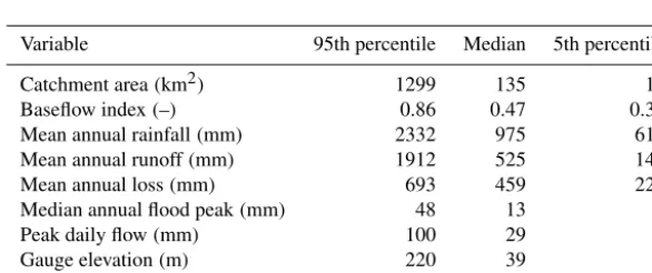
Table 1.Characteristics of the 1013 catchments included in this study. Values for mean annual rainfall, runoff, loss, flood peaks and peak daily flows were calculated from the model input time series. Other values were taken from the UK hydrometric register (Marsh and Hannaford, 2008b).

Variable 95th percentile Median 5th percentile Catchment area(km2) 1299 135 17 Baseflow index(–) 0.86 0.47 0.30 Mean annual rainfall(mm) 2332 975 618 Mean annual runoff(mm) 1912 525 146 Mean annual loss(mm) 693 459 220 Median annual flood peak(mm) 48 13 2 Peak daily flow(mm) 100 29 4 Gauge elevation(m) 220 39 5 Urban extent(%) 19 1 0

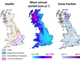
On average, rainfall is highest in the north and west of GB, and lowest in the south and east, with GB totals varying from a minimum of 500 mm to a maximum of 4496 mm per year (see Fig. 2). There is also seasonal variation, with the highest monthly rainfall totals generally occurring dur-ing the winter months and the lowest totals occurrdur-ing in the summer months. This pattern is enhanced by seasonal varia-tions in temperature, with evaporation losses concentrated in the summer months from April–September. Besides climatic conditions, river flow patterns are also heavily influenced by groundwater contributions. Figure 1 shows the major aquifers in GB. In catchments overlying the Chalk outcrop in the south-east, flow is groundwater-dominated with a pre-dominantly seasonal hydrograph that responds less quickly

to rainfall events. Land use and human modifications to river flows also significantly impact river flows, with river flows being heavily modified in the south-east and midland regions of England due to high population densities (Fig. 1). Most catchments have very little or no snowfall in an average year, but there are some upland catchments in northern England and north-eastern Scotland where up to 15 % of the annual precipitation falls as snow (Fig. 2).

Figure 2. (a)Major aquifers across Great Britain, based on BSS Geology 625k, with the permission of the British Geological Survey.

(b)Mean annual rainfall for 10 km2rainfall grid cells across Great Britain.(c)Fraction of rainfall falling as snow for catchments across Great Britain, where a value of 0.15 indicates that 15 % of the catchment precipitation falls on days when the temperature is below zero.

1013 had sufficient information (defined as more than 10 years of available discharge data during the model evaluation period of 1993–2008) available to include in this analysis.

2.2 Observational data

Twenty-one years of daily rainfall and PET data covering the period 1 January 1988 to 31 December 2008 were used as hydrological model input. Rainfall time series were derived from the Centre for Ecology and Hydrology Gridded Esti-mates of Areal Rainfall, CEH-GEAR (Tanguy et al., 2014). This is a 1 km2 gridded product giving daily estimates of rainfall for Great Britain (Keller et al., 2015). It is based on the national database of rain gauge observations collated by the UK Met Office, with the natural neighbour interpolation methodology used to convert the point data to a gridded prod-uct (Keller et al., 2015).

The Climate Hydrology and Ecology research Support System Potential Evapotranspiration (CHESS-PE) dataset was used to estimate daily PET for each catchment. The CHESS-PE dataset is a 1 km2 gridded product for Great Britain, providing daily PET time series (Robinson et al., 2015a). PET estimates were produced using the Penman– Monteith equation, calculated using meteorological vari-ables from the CHESS-met dataset (Robinson et al., 2015b). Catchment areal daily precipitation and PET time series were produced for each catchment by averaging values of all grid

squares that lay within the catchment boundaries for each of the 1013 catchments.

Observed discharge data were used to evaluate model per-formance. Gauged daily flow data from the NRFA were used for all catchments where available (Centre for Ecology and Hydrology, 2016).

3 Methodology

3.1 Hydrological modelling

The FUSE modelling framework was used to provide four al-ternative hydrological model structures. This framework was selected as it enables comparison between hydrological mod-els with varying structural components (Clark et al., 2008), and the computational efficiency of these relatively simple hydrological models enabled modelling to be carried out across a large number of catchments within an uncertainty analysis framework. The framework allows the user to select different combinations of modelling decisions, starting with four parent models based on the structures of widely used hydrological models and allowing the user to combine these decisions to create over 1000 different model structures.

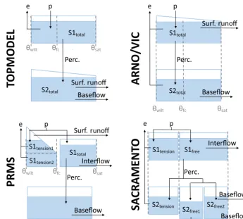
Figure 3.FUSE wiring diagram, showing the model structure decisions. TOPMODEL and ARNO/VIC have 10 parameters, PRMS has 11 parameters, and SACRAMENTO has 12 parameters. Adapted from Clark et al. (2008).

the core differences of models compared to all the possible variants. These models are based on four widely used hydro-logical models: TOPMODEL (Beven and Kirkby, 1979), the Variable Infiltration Capacity (ARNO/VIC) model (Liang et al., 1994; Todini, 1996), the Precipitation-Runoff Modelling System (PRMS; Leavesley et al., 1983) and the SACRA-MENTO model (Burnash et al., 1973). The models are all lumped, conceptual models of similar complexity and all run at a daily time step within the FUSE framework. They all close the water balance, have a gamma routing function and include the same processes; for example, none of the mod-els have a snow routine or vegetation module. However, the structures of these models differ through the architecture of the upper and lower soil layers and parameterisations for sim-ulation of evaporation, surface runoff, percolation from the upper to lower layer, interflow and baseflow (Clark et al., 2008), as shown in Fig. 3 and Table 3. This leads us to be-lieve that the model structures are dynamically different, as they represent hydrological processes in different ways, yet as all are based on widely used hydrological models, they are equally plausible. Therefore we have no a priori expectations that one model should outperform the others (Clark et al., 2008).

The models were run within a Monte Carlo simulation framework. There are 23 adjustable parameters within the FUSE framework, as shown in Table 2. Each of these was as-signed upper and lower bounds based on feasible parameter ranges and behavioural ranges identified in previous research (Clark et al., 2008; Coxon et al., 2014). Monte Carlo sam-pling was then used to generate 10 000 parameter sets within these given bounds. Therefore, for each of the 1013 catch-ments, the four hydrological model structures were each run using the 10 000 possible parameter sets over the 21-year pe-riod 1988–2008, resulting in>40 million simulations being carried out.

3.2 Evaluation of model performance

Table 2.FUSE parameters and defined upper and lower bounds.

Parameter Description Units Lower Upper Model(s) using parameter

bound bound

MAXWATER 1 Depth of upper soil layer mm 25 500 TOPMODEL, ARNO, PRMS, SACRAMENTO

MAXWATER 2 Depth of lower soil layer mm 50 5000 TOPMODEL, ARNO, PRMS, SACRAMENTO

FRACTEN Fraction total storage in tension storage – 0.05 0.95 TOPMODEL, ARNO, PRMS, SACRAMENTO FRCHZNE Fraction tension storage in recharge zone – 0.05 0.95 PRMS

FPRIMQB Fraction storage in first baseflow reservoir – 0.05 0.95 SACRAMENTO

RTFRAC1 Fraction of roots in the upper layer – 0.05 0.95 ARNO

PERCRTE Percolation rate mm d−1 0.01 1000 TOPMODEL, ARNO, PRMS

PERCEXP Percolation exponent – 1 20 TOPMODEL, ARNO, PRMS

SACPMLT SACRAMENTO model percolation multiplier for dry soil layer – 1 250 SACRAMENTO SACPEXP SACRAMENTO model percolation exponent for dry soil layer – 1 5 SACRAMENTO PERCFRAC Fraction of percolation to tension storage – 0.5 0.95 SACRAMENTO

FRACLOWZ Fraction of soil excess to lower zone – 0.5 0.95 PRMS

IFLWRTE Interflow rate mm d−1 0.1 1000 PRMS, SACRAMENTO

BASERTE Baseflow rate mm d−1 0.001 1000 TOPMODEL, ARNO

QB_POWR Baseflow exponent – 1 10 TOPMODEL, ARNO

QB_PRMS Baseflow depletion rate d−1 0.001 0.25 PRMS

QBRATE_2A Baseflow depletion rate first reservoir d−1 _{0.001 0.25 SACRAMENTO}

QBRATE_2B Baseflow depletion rate second reservoir d−1 0.001 0.25 SACRAMENTO

SAREAMAX Maximum saturated area – 0.05 0.95 PRMS, SACRAMENTO

AXV_BEXP ARNO/VICbexponent – 0.001 3 ARNO

LOGLAMB Mean value of the topographic index m 5 10 TOPMODEL

TISHAPE Shape parameter for the topographic index gamma distribution – 2 5 TOPMODEL

TIMEDELAY Time delay in runoff d 0.01 7 TOPMODEL, ARNO, PRMS, SACRAMENTO

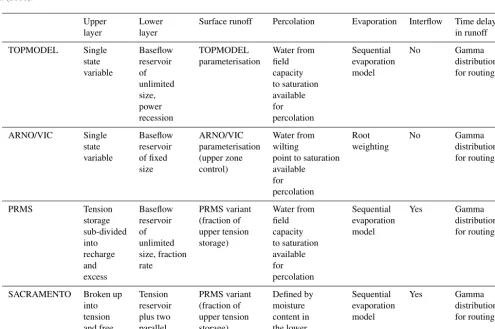
Table 3.Modelling decisions in the four parent models of the FUSE framework. A full description of the models can be found in Clark et al. (2008).

Upper Lower Surface runoff Percolation Evaporation Interflow Time delay

layer layer in runoff

TOPMODEL Single Baseflow TOPMODEL Water from Sequential No Gamma state reservoir parameterisation field evaporation distribution variable of capacity model for routing

unlimited to saturation size, available

power for

recession percolation

ARNO/VIC Single Baseflow ARNO/VIC Water from Root No Gamma state reservoir parameterisation wilting weighting distribution variable of fixed (upper zone point to saturation for routing

size control) available for percolation

PRMS Tension Baseflow PRMS variant Water from Sequential Yes Gamma storage reservoir (fraction of field evaporation distribution sub-divided of upper tension capacity model for routing into unlimited storage) to saturation

recharge size, fraction available

and rate for

excess percolation

SACRAMENTO Broken up Tension PRMS variant Defined by Sequential Yes Gamma into reservoir (fraction of moisture evaporation distribution tension plus two upper tension content in model for routing and free parallel storage) the lower

models through the widely used Nash–Sutcliffe efficiency in-dex (Nash and Sutcliffe, 1970), which is an easy-to-interpret measure of model performance that is often used in studies interested in high flows, as it emphasises the fit to peaks. To further diagnose the reasons for model good or poor perfor-mance, the simulation with the highest efficiency value was then analysed further using the decomposed metrics of bias, error in the standard deviation and correlation.

All metrics were calculated for the period 1993–2008, with the first 5 simulation years being used as a model warm-up period.

The Nash–Sutcliffe efficiency index was calculated for each individual simulation using

E=1− P

(Oi−Si)2 P

Oi−O

2, (1)

whereOi refers to the observed discharge at each time step,

Si refers to the simulated discharge at each time step and ¯

Ois the mean of the observed discharge values. This results in values ofEbetween 1 (perfect fit) and−∞, where a value of zero means that the model simulation has the same skill as using the mean of the observed discharge.

To gain insights into model agility and time-varying model performance during different times of the year, we also as-sessed differences in seasonal performance by splitting the observed and simulated discharge into March–May (spring), June–August (summer), September–November (autumn) and December–February (winter). Seasonal Nash–Sutcliffe effi-ciency values were then re-calculated for all the catchments, using only data extracted for that season. This allowed us to see if there were any seasonal patterns in model performance, for example during periods of higher or lower general flow conditions.

The Nash–Sutcliffe efficiency can be decomposed into three distinct components: the correlation, bias and a mea-sure of the error in predicting the standard deviation of flows (Gupta et al., 2009). Understanding how the models perform for these different components can help us diagnose why models are producing good or poor simulations. We there-fore calculated these simpler metrics for the simulations of each model gaining the highest efficiency values. The rela-tive bias was calculated using

µ=µs−µo

µo

, (2)

whereµs andµorefer to the mean of the simulated and

ob-served annual cycle. Using this equation, an unbiased model would score 0 (a perfect score) and a model that underesti-mated or overestiunderesti-mated the mean annual flow would score a negative or positive value respectively. A value of±1 would indicate an overestimation or underestimation of flow by 100 %.

The relative difference in the standard deviation was cal-culated using

σ=σs−σo

σo

, (3)

whereσsandσorepresent the standard deviation of the

simu-lated and observed mean annual cycle. Again, a value of zero indicates a perfect score with no error, and positive or nega-tive values indicate an overestimation or underestimation of the amplitude of the mean annual cycle respectively.

The correlation was calculated using Pearson’s correlation coefficient. A value of 1 indicates a perfect correlation be-tween the observed and simulated flows, whilst a value of 0 indicates no correlation. This indicates model skill in captur-ing both timcaptur-ing and shape of the hydrograph.

3.3 Evaluation of model predictive capability

In order to evaluate model predictive capability, the widely applied GLUE framework was used (Beven and Freer, 2001; Romanowicz and Beven, 2006). The GLUE framework is based on the equifinality concept that there are many differ-ent model structures and parameter sets for a given model structure which result in acceptable model simulations of observed river flow (Beven and Freer, 2001). This method-ology has been widely applied to explore parameter uncer-tainty within hydrological modelling (Freer et al., 1996; Gao et al., 2015; Jin et al., 2010; Shen et al., 2012) and includes approaches to directly deal with observational uncertainties in the quantification of model performance (Coxon et al., 2014; Freer et al., 2004; Krueger et al., 2010; Liu et al., 2009). For every catchment and model structure, an effi-ciency score was calculated for each of the 10 000 Monte Carlo (MC) sampled parameter sets. Parameter sets with an efficiency score exceeding 0.5 were regarded as behavioural; therefore all other sampled parameter sets were rejected and so given a score of zero. Conditional probabilities were as-signed to each behavioural parameter set based on their be-havioural efficiency score, and these were normalised to sum to 1. This meant that the simulations which scored the high-est efficiency value had larger conditional probabilities, and simulations which had efficiency values just above 0.5 would have lower conditional probabilities. For each daily time step, a 5th, 50th and 95th simulated discharge bound was pro-duced from these conditional probabilities, for each catch-ment and model structure individually, as described in Beven and Freer (2001). This meant that simulations with a higher efficiency score were given a higher weighting when produc-ing the discharge bounds.

sim-ulated discharge uncertainty bounds. Two metrics were then used to assess the predictive capability of the models. The first metric aimed to assess the model’s ability to closely replicate the observed annual maximum flows whilst con-sidering the plausible range of observational uncertainties that may be associated with the observed discharge value. Observed uncertainty bounds of ±13 % were applied to all observed annual maximum (AMAX) discharges. This ob-served error value was selected following previous research on quantifying discharge uncertainty at 500 UK gauging stations for high flows and represents the average 95th-percentile range of the discharge uncertainty bounds for high flows (Coxon et al., 2015; Mcmillan et al., 2012). The equa-tions used to calculate the model skill relative to these obser-vational uncertainty bounds are

Ey= Oy−Sy

Oy×0.13

, (4)

Emean= n P

y=1

Ey

n , (5)

where Ey refers to skill for a particular year, y, Emean

refers to skill across all years,O refers to observed AMAX discharge for a particular year andSrefers to the simulated AMAX discharge for the 50th percentile. This results in a score of 0 if the AMAX that is simulated for the 50th per-centile is equal to observed AMAX discharge, a score of 1 if the simulated AMAX is at the limit of the observed error bounds, and a score of 2 if it is twice the limit and so on in a similar approach to Liu et al. (2009) as a limits of acceptabil-ity performance score. A score was calculated for each of the 16 simulation years, excluding the first 5 years as a model warm-up period, as shown in Eq. (4). A mean score was then calculated across all years for each catchment and model, as shown in Eq. (5).

The second metric assessed how well the simulated AMAX uncertainty bounds (5th to 95th) overlapped ob-served AMAX uncertainty bounds to assess model skill given the range of predictive uncertainty. The range of overlap be-tween the observed discharge uncertainty bounds and sim-ulated bounds was first calcsim-ulated for each year. This was normalised by the maximum range of the observed and sim-ulated AMAX uncertainty bounds. The resulting value can be interpreted as the fraction of overlap versus the total uncer-tainty, whereby a value of 0 means that the simulated AMAX bounds for a particular year do not overlap the observations at all, and a value of 1 means that the simulated bounds perfectly overlap the observational uncertainties. Therefore, simulation bounds which overlap the observed AMAX un-certainty range due to having a very large unun-certainty spread are penalised for this additional uncertainty width compared to the observed normalised uncertainty.

4 Results

4.1 National-scale model performance

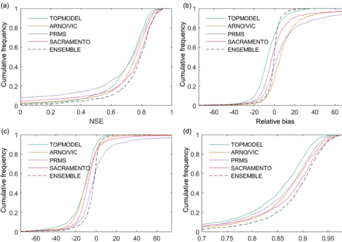
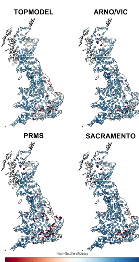
Our first objective was to assess how well simple, lumped hy-drological model structures perform across Great Britain, as-sessed over annual timescales via standard performance met-rics. The distributions of model performance across all catch-ments can be seen in Fig. 4. This shows that the ensemble of all four hydrological model structures outperformed each in-dividual model structure for all performance metrics. Using the ensemble, 93 % of catchments studied produced a simula-tion with a Nash–Sutcliffe efficiency (NSE) value exceeding 0.5, and 75% of catchments exceeded an NSE value of 0.7. Maps showing the overall performance of each model struc-ture, chosen using the maximum modelled NSE from the MC parameter samples, for catchments across Great Britain are given in Fig. 5. Maps showing the performance of each model structure for the other performance metrics are given in Fig. 6.

Our NSE results (Figs. 4 and 5) show that there is a large range in model performance across Great Britain, with catch-ment maximum NSE scores ranging from 0.97 to<0. The overall performance of the four model structures was simi-lar, with TOPMODEL, ARNO, PRMS and SACRAMENTO producing simulations exceeding a 0.5 NSE for 87 %, 90 %, 81 % and 88 % of catchments respectively. A similar spatial pattern of performance was also seen across all four model structures, with certain catchments resulting in poor or good simulations for all four model structures. Generally, there is an east–west divide in model performance, with models typically performing better in the wetter western catchments compared to drier catchments in the east. Clusters of poorly performing catchments can be seen in the east of England around London and in central Scotland, where all models fail to produce satisfactory simulations. There are also more lo-calised catchments where all models are failing, such as in north Wales and northern England. Areas where all models are performing well include southern Wales, south-western England and south-western Scotland.

partic-Figure 4.Distribution of model performance across all catchments for all four individual model structures and the model structure ensemble. Each plot shows model performance assessed using a different metric.(a)shows model performance assessed using Nash–Sutcliffe efficiency,

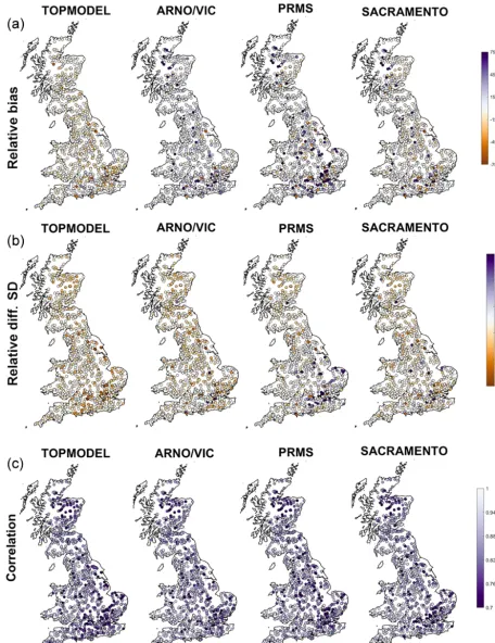
(b)shows model relative bias or relative error in simulated mean runoff (%),(c)shows relative error in the standard deviation of runoff (%), and(d)gives correlation between observed and simulated streamflow.

ularly interesting that whilst the models are all calibrated in the same way and are producing similar NSE scores, the de-composed metrics show clear differences between the best simulations produced using each structure.

The decomposed metrics also help to identify which as-pects of NSE are causing models to fail. Models have prob-lems simulating the bias, standard deviation and correlation for catchments in south-eastern England (Fig. 6). The lo-calised poorly performing catchments in north Wales are fail-ing due to poor simulation of variance and correlation. Poor performance in north-eastern Scotland is due to poor correla-tion and underestimacorrela-tion of variance for all models. In cen-tral northern Scotland all models except TOPMODEL over-predict bias, leading to TOPMODEL being the only model able to produce reasonable simulations for these catchments. Similarities in overall model performance could be par-tially due to the models all being run at the same spatial and temporal resolution, having a similar model architecture splitting the catchment into upper and lower stores and in-cluding the same process representations (such as a lack of a snow module). However, there are important differences between the models which may contribute to the differences seen in the decomposed metrics (Fig. 6). The architecture of the upper and lower model layers differs, as can be seen in Fig. 3. TOPMODEL and ARNO/VIC have more parsi-monious structures with only one store in each layer, while PRMS has a more complex upper layer which is split into multiple stores, and SACRAMENTO splits both upper and

lower layers into multiple stores. The modelling equations governing water movement between stores also differ, as ex-plained in Clark et al. (2008). The number of model parame-ters is also a difference between the models, as shown in Ta-ble 2, with TOPMODEL and ARNO/VIC having the fewest model parameters, with 10 model parameters each, and the SACRAMENTO model having the most parameters, with 12.

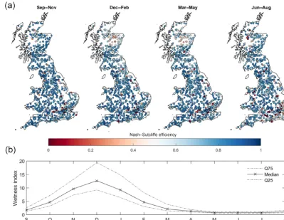
4.2 Seasonal model performance

As part of our first objective, we also assessed how well models performed across GB when evaluated over seasonal timescales, with results given in Fig. 7. These maps show the best sampled seasonal NSE score for each catchment taken from any of the FUSE model variants. There is a clear sea-sonal pattern to model performance, with models generally producing better simulations during wetter winter periods. The models cannot produce adequate simulations for many catchments over the summer months of June to August, espe-cially in the south-east of England. However, for some catch-ments, especially catchments in the west, good simulations are produced year-round.

sim-Figure 5.GB maps of model performance for each structure. Each point is a gauge location which is coloured based on the best Nash– Sutcliffe score attained by the model for that catchment.

ulated in summer. In south-eastern England, model perfor-mance is particularly poor during the summer months of June–August. The reasons for this are discussed in later sec-tions.

4.3 Model structure impact on performance

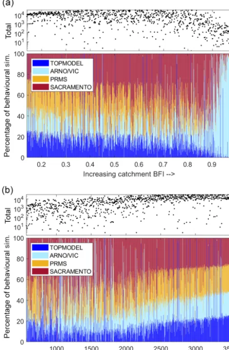
An interesting question is whether a certain model structure is favoured for certain types of climatology or generalised catchment behaviour. Therefore, the relative performance of the four model structures, ranked by both the baseflow in-dex (BFI) and annual catchment rainfall totals, is presented in Fig. 8. The SACRAMENTO model tends to be the domi-nant model structure across most catchments, producing the

largest number of behavioural simulations. However, catch-ment BFI and annual average rainfall both have an impact on which model structure tends to produce the most behavioural simulations as well as the total number of behavioural simu-lations.

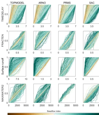
Catchments with an increasing BFI from 0 to 0.87 show an increasing trend of the SACRAMENTO model struc-ture becoming dominant, albeit with considerable variabil-ity (see Fig. 8a). TOPMODEL and PRMS performance rel-ative to the other models decreased for catchments with increasing BFI, and TOPMODEL especially is known to have a conceptual structure that better relates to a variable source area concept that does not relate as well to more groundwater-dominated catchments. However, for slower re-sponding and more groundwater-dominated catchments with a BFI of greater than 0.9, the ARNO/VIC model was the only structure able to represent the hydrological dynamics well. ARNO/VIC is the only model that has a very strong non-linear relationship in its upper storage zone that links the deficit ratio of this store to saturated area extent and thus rainfall-driven surface runoff amounts. For very low values of the ARNO/VIC “b” exponent (AXV_BEXP), as seen for high BFI values in Fig. 9 for behavioural model distributions, means that only at very high, near-full upper storage levels is any larger extent of saturated areas predicted. This for-mulation clearly helps these more groundwater-dominated catchments where both higher infiltration and percolation dy-namics may be expected by constraining fast rainfall-driven runoff processes except to only more extreme storm event be-haviour. It is also the reason why the sensitivity to BFI of this parameter is stronger in Fig. 9 than the other “surface runoff” formulations that link storages to saturated area extent.

Figure 7.GB maps of FUSE multi-model ensemble model performance for each season(a)and observed seasonal variations in catchment wetness index(b). Each point in(a)is a gauge location which is coloured based on the best Nash–Sutcliffe score attained by any of the four models sampled for that catchment and season.(b)then shows how seasons vary hydrologically across GB, through the wetness index (precipitation/PET or precipitation divided by PET) calculated from the observed data, split by month, used to drive the hydrological models across all catchments shown in(a).

4.4 Influence of hydrological regime and catchment attributes on model performance

The influence of the hydrological regime was then assessed to see if there were specific types of catchments that the mod-els were unable to represent given the spatial differences in model performance already observed. The catchment hydro-logical regime was defined using two metrics, the overall runoff coefficient (ratio of annual discharge to annual rain-fall) and the catchment wetness index (ratio of precipita-tion to potential evapotranspiraprecipita-tion); results are provided in Fig. 10. The relationship between model performance and a wider range of catchment characteristics is given in the Sup-plement.

Figure 10 shows that model performance relates to the catchment water balance. For catchments where the water balance tends to close, indicated as the area between the dashed lines, the models are generally able to produce rea-sonable simulations overall and with small biases. For these catchments, precipitation, evaporation and discharge are bal-anced, and runoff can be explained using the precipitation

Figure 8.Relative performance of the four FUSE model structures, depending on catchment characteristics. Scatter plots show the to-tal number of behavioural simulations, from all model structures, forming each line on the stacked bar graph. Each line on this stacked bar chart represents one catchment, and the colour shows the pro-portion of the behavioural simulations from each model structure. Catchments have been ordered by BFI(a)and annual rainfall(b).

4.5 Benchmarking predictive capability for annual maximum peak flows

Model predictive capability for simulating AMAX flows from behavioural models defined from the NSE measure is shown in Figs. 11 and 12. Figure 11 assesses the ability of models to produce AMAX discharge estimates which are as close as possible to observations. Here, a value of 0 means that simulated AMAX discharge is equal to observed dis-charge, up to 1 means that simulated AMAX discharge is within the bounds of the observational uncertainties applied and larger values such as 2 indicate that simulated discharge is double the limit of observational uncertainties away from the observed discharge (negative values mean that the model simulations are lower than the observed). MedianEamax

val-ues from Eq. (2) are around−2.4 to −3.2 across all four models, with PRMS producing slightly better predictions in general than the other models. This shows that the models underestimate peak annual discharges across the majority of GB catchments even though behavioural models have been selected using NSE, which favours models that perform well for higher flows.

Figure 12 shows the percentage overlap between the sim-ulated 5th and 95th AMAX bounds and the observed AMAX uncertainty bounds. Here, the boxplot on the left shows the variation of results across all catchments and models for each year, whilst the boxplot on the right summarises results across all catchments and years for each model. The median value across all catchments is 16, meaning that there is a 16 % overlap between the observed and simulated AMAX bounds averaged across all 20 years.

There are large variations in model ability to simulate ob-served annual maximum flows between years when looking at median predictions. For example, 1990 and 2008, which were wetter-than-average years across most of GB, model ability to represent annual maximum discharge is poor. How-ever, in 1996, which was a particularly dry year following the 1995 drought (Marsh et al., 2007), the models do a much bet-ter job of representing the annual maximum discharge. This may be in part due to the model tendency to underestimate discharge, as seen in Fig. 11. However, variations between years are less apparent when looking at 25th and 75th per-centiles in Fig. 12. This could suggest that there are some catchments where predictions are more consistent between years or that the large climatic variation across GB may con-ceal some of the effects of inter-year differences.

5 Discussion

This study provides a useful benchmark of the performance and associated uncertainties of four commonly used lumped model structures across GB for future model developments and model types to be compared against. The large num-ber of catchments included makes this assessment a fair benchmark for any future national modelling studies as well as for smaller-scale modelling efforts. A full list of models scores can be found at https://doi.org/10.5523/bris. 3ma509dlakcf720aw8x82aq4tm.

Figure 9.Cumulative distribution function (CDF) plots showing parameter values of the behavioural simulations for each catchment. Each line represents a catchment and is coloured by that catchment’s BFI. The four rows show different parameters controlling different parts of the hydrograph. Surface runoff is given by the LOGLAMB (TOPMODEL), AXV_BEXP (ARNO) and SAREAMAX (PRMS and SACRA-MENTO), as there was no common surface runoff parameter used for all four models. Each column is a different hydrological model.

north-eastern Scotland are classed as natural, but there are a group of catchments in central northern Scotland which are impacted by hydro-electric power (HEP) generation and subsequent diversions out of the catchment as well as stor-age influences on the regime (Marsh and Hannaford, 2008b). As model failures in north-eastern Scotland were particularly pronounced during winter and spring, this suggests that mod-els were unable to capture the different seasonal climatic con-ditions of these catchments, such as snow accumulation and melt or the impact of frozen ground. This is supported by the low correlations between simulated and observed flows in north-eastern Scotland, suggesting that the models are un-able to represent the overall shape and timing of flows. Many catchments in central and northern Scotland had particularly low NSE values which were worst in summer and autumn.

Modifications to the flow regime resulting from HEP can explain poor model performance for these catchments, sup-ported by the models failing to reflect model bias and correla-tion. The FUSE models in this study do not incorporate snow processes and indicate that future modelling efforts for GB may need to include a snowmelt regime, and the anthro-pogenic impacts resulting from hydroelectric power gener-ation, to produce good simulations in these catchments.

Figure 10.Scatter plots of the relationship between wetness index, runoff coefficient and best sampled model performance. Each point represents a catchment, coloured by the best Nash–Sutcliffe score for that catchment from the model structure ensemble. The plotting order was modified to ensure that catchments with more extreme (high and low) performance values would be plotted on top. Any points above the horizontal dotted line are where runoff exceeds total rainfall in a catchment, and any points below the curved line are where runoff deficits exceed total PET in a catchment.(a)is coloured by Nash–Sutcliffe efficiency, and(b–d)are coloured by relative bias, relative error in the standard deviation, and correlation between simulated and observed streamflow.

of the chalk aquifer could also stress the models, as there is nothing in the model structures to account for groundwa-ter and particularly groundwagroundwa-ter flows between catchment boundaries. Equally, the south-east has some of the high-est population densities in the UK, and human influences can significantly impact flows in this region, particularly for lower-flow conditions in the drier seasonal periods.

Figure 11.Predictive capability of four hydrological models for annual maximum (AMAX) flows across Great Britain. Shown is behavioural model ensemble (NSE>0.5) median performance in replicating the observed AMAX flows, with a value of 0 being a perfect score and a value of 1 meaning that the simulated AMAX value was at the limits of the observational uncertainty. The spread covers all catchments.

Figure 12.Predictive capability of four hydrological models for an-nual maximum (AMAX) flows across Great Britain. Boxplots show the overlap of the simulated and observed uncertainty bounds, as a percentage of the total uncertainty. This metric ranges from 0 to 100, with 0 indicating no overlap between observed and simu-lated AMAX discharge and 100 indicating a perfect overlap of ob-served and simulated discharge bounds. The range in the(a)is over all catchments and all models, whilst(b)shows the range across all catchments.

has been noted that there is a general pattern of poor per-formance for catchments in south-eastern England, it is hard to disentangle the reasons why this may be the case. Both the underlying chalk geology causing water transfer between catchments and heavily human-modified flow regimes could explain model failures which are greatest during the sum-mer. Interestingly, McMillan et al. (2016) found that whilst the aquifer fraction was expected to have a strong link to model performance, no relationship was found for the TOP-NET model applied in New Zealand.

5.2 Influence of catchment characteristics and climate on model performance

One of the key advantages of large-sample studies is that by applying models to many catchments, we can see general trends and identify important catchment characteristics or climates that are not represented well by our choice of model structures. We found that looking at the catchment water bal-ance, considering the relationship between catchment pre-cipitation, evaporation and observed flows, helped to iden-tify common features of catchments where all models were failing (Figs. 5 and 10). All model structures produced poor simulations in catchments where either total runoff exceeded total rainfall or where observed runoff was very low com-pared to total rainfall, and this runoff deficit could not be ac-counted for by evapotranspiration losses alone. These differ-ences in water balance are likely due to human modifications to the natural flow regime, such as dams, effluent returns, or inter-catchment water transfers or groundwater flow between catchments, or it is also possible that there are systematic er-rors in the observational data and that this information is dis-informative (Beven and Westerberg, 2011; Kauffeldt et al., 2013). Most of these catchments were located within chalk aquifers in south-eastern England and therefore are in a heav-ily urbanised area where groundwater abstractions and flows between catchments could be expected. The simple, lumped models used here were only given inputs of observed pre-cipitation and PET; therefore they are unable to account for the additional observed runoff and so are “stressed”, even in terms of simulating mean annual runoff, irrespective of more detailed hydrograph behaviour.

We also found that catchment characteristics were impor-tant in determining which model structure was most appro-priate. For catchments with a high baseflow index, only the ARNO/VIC model was able to produce behavioural simula-tions. This could be explained by the strong non-linear rela-tionship in the upper storage zone of the ARNO/VIC model, which separates it from the other model structures. This en-ables the ARNO/VIC model to constrain the fast rainfall– runoff processes, which would only occur for extreme events in these groundwater-dominated catchments and so allow for a complex mixture of highly non-linear saturated fast re-sponses coupled with more general baseflow dynamics to be captured effectively. The catchment annual rainfall total

also influenced which model structure was most appropri-ate. We found that for catchments with average annual rain-fall values of around 2000 mm yr−1 _{or lower, the}

SACRA-MENTO model structure is more dominant. As we move to-wards catchments with higher annual rainfall, the relative im-portance of the different structures shift until all structures are approximately equal for the catchments with the highest annual rainfalls. This shows that for very wet catchments, the model structure is less important, as all models can produce behavioural simulations through some part of the parameter space, as seen by the relatively high number of behavioural simulations for wetter catchments (Fig. 8b). This agrees with previous studies, where models have been found to perform better for wetter catchments, which are likely to have more connected saturated areas, as there is a more direct link be-tween rainfall and runoff (McMillan et al., 2016).

Our results highlight the difficulty in national and large-scale modelling studies, which for GB must incorporate human-modified hydrological regimes, complex groundwa-ter processes, a range of different climates and the poten-tial of dis-informative data, or at least a lack of process un-derstanding to adjust model conceptualisations. Whilst ple, lumped hydrological models can produce adequate sim-ulations for most catchments, the model structures are put under too much stress when trying to simulate catchments where the water balance does not close or is increasingly de-parting from normal conditions. The models fail or produce poor simulations when large volumes of water enter or leave the catchment due to human activities or groundwater pro-cesses, indicating the importance of considering these influ-ences in any national study. What is striking here in these results is that general hydrological processes, defined by wa-ter availability and BFI metrics to infer the extent of slower flow pathways, are important in defining the quality of sim-ulated output and differences in model structures and param-eter ranges even though nationally many catchments are im-pacted by additional anthropogenic activities such as abstrac-tions and multiple flow structures.

5.3 Predictive capability of models for predicting annual maximum flows

maxi-mum flows. Newman et al. (2015) found the same effect in their study covering 617 catchments across the US. This un-derestimation of peaks could be in part due to the use of NSE in selection of the behavioural models. NSE is often used in flood studies, as it emphasises correct prediction of flood peaks relative to low flows (for example, Tian et al., 2013). However, NSE tends to underestimate the overall variance in the time series, resulting in underprediction of floods and overprediction of low flows (Gupta et al., 2009).

It was found that there were some variations in the abil-ity of models to simulate AMAX flows between years, and this often related to the wetness of a particular year. Models tended to perform worse in wetter years and better in drier years. This could be linked to the fact that all models tended to underestimate annual maximum flows and therefore are closer to observations in years with lower annual maximum flows.

5.4 Uncertainty evaluation in hydrological modelling This study evaluated both model parameter and model struc-tural uncertainty. The results showed that there is consid-erable value in using multiple model structures. No one model structure was appropriate for all catchments or sea-sons and when evaluating different metrics from the hydro-graphs. We found that generally the SACRAMENTO model resulted in the best NSE values overall, TOPMODEL was able to produce the simulations with the least biases and the ARNO/VIC model proved to be best for high baseflow catchments, though the PRMS model was the best at cap-turing AMAX peak flows. Furthermore, it was found that for some catchments only a selection of the model structures were able to produce good simulations, such as the baseflow-dominated catchments which only ARNO/VIC could simu-late well. For these catchments, selection of the appropriate model structure is important for producing good simulations, and unsuitability of the model structure cannot be corrected for through parameter calibration. This supports previous re-search highlighting the importance of considering alterna-tive model structures and using model structure ensembles or flexible frameworks such as FUSE (Butts et al., 2004; Clark et al., 2008; Perrin et al., 2001). Consequently, future hydro-logical modelling over a national scale and/or over a large sample of catchments needs to ensure that appropriate model structures are selected for these catchments and consider the possibility of using multiple model structures to represent hy-drological processes in varied catchments.

The results also highlighted the importance of consider-ing parameter uncertainty. It was shown that there were of-ten many different parameter sets which could produce good simulation results for the same model structure. For some catchments, particularly the wetter catchments in the west, all model structures were able to produce good simulations through sampling the parameter space. We also show how behavioural parameter distributions change with regards to

the BFI (Fig. 9), which shows expected shifts in some of the common behavioural parameters or concepts for different conditions, showing that the model behaviour and parameter formulations are in general making rational sense (i.e. higher BFI equals higher time delays).

While this study incorporated uncertainties in model struc-tures and parameters, future work will also focus on incor-porating uncertainties in the data used to drive hydrological models and more sophisticated representation of discharge uncertainties. This is important because errors in observa-tional data will introduce errors to runoff predictions when fed through rainfall–runoff models (Andréassian et al., 2001; Fekete et al., 2004; Yatheendradas et al., 2008), and in con-junction with uncertainties in the observational data used to evaluate hydrological models, they will also affect our abil-ity to calibrate and evaluate hydrological models (Blazkova and Beven, 2009; Coxon et al., 2014; McMillan et al., 2010; Westerberg and Birkel, 2015).

6 Summary and conclusions

In this study, we have benchmarked the performance of an ensemble of lumped, conceptual models across over 1000 catchments in Great Britain.

Overall, we found that the four models performed well over most of Great Britain, with each model producing simu-lations exceeding a 0.5 Nash–Sutcliffe efficiency over at least 80 % of catchments. The performance of the four models was similar, with all models showing similar spatial patterns of performance and no single model outperforming the others across all catchment characteristics for both daily flows and peak flows. However, when decomposing NSE into model performance for bias, standard deviation error and correla-tion, clear differences emerged between the best simulation produced by each of the model structures. The ensemble did better than each individual model, demonstrating the value of model structure ensembles when exploring national-scale hydrology.

We found that all models showed higher skill in simulating the wet catchments to the west, and all models failed in ar-eas of Scotland and south-ar-eastern England. Sar-easonal perfor-mance and analysis of the water balance suggested that these model failures could be at least in part attributed to miss-ing snowmelt or frozen ground processes in Scotland and chalk geology in south-eastern England, where water was able to move between catchment boundaries. In general, we found that models performed poorly for catchments with un-accounted losses or gains of water, which could be due to measurement errors, water transfer between catchments due to groundwater aquifers and human modifications to the wa-ter system. Therefore, these factors would need to be consid-ered in a national model of Great Britain.

hy-drograph, assessed using Nash–Sutcliffe efficiency, does not necessarily mean that models are performing well for other hydrological signatures. We found that the FUSE models tended to underestimate peak flows, and there were variations in model ability between years, with models performing par-ticularly poorly for extremely wet years.

This benchmark series provides a useful baseline for as-sessing more complex modelling strategies. From this we can resolve how or where we can and need to improve mod-els to understand the value of different conceptualisations, linkages to human impacts and levels of spatial complexity that our model frameworks could deploy in the future. There-fore, the results of this study are made available at https: //doi.org/10.5523/bris.3ma509dlakcf720aw8x82aq4tm.

Code availability. FUSE model code is introduced in Clark et al. (2008) and is available upon request from the lead author.

Data availability. All datasets used in this study are pub-licly available. The CEH-GEAR and CHESS-PE datasets are freely available from CEH’s Environmental Information Data Centre and can be accessed through https://doi.org/10.5285/ 5dc179dc-f692-49ba-9326-a6893a503f6e (Tanguy et al., 2014) and https://doi.org/10.5285/8baf805d-39ce-4dac-b224-c926ada353b7 (Robinson et al., 2015a) respectively. Observed discharge data from the NRFA are available from the NRFA website. All model output data produced for this paper are avail-able at the University of Bristol data repository, data.bris, at https://doi.org/10.5523/bris.3ma509dlakcf720aw8x82aq4tm.

Supplement. The supplement related to this article is available on-line at: https://doi.org/10.5194/hess-23-4011-2019-supplement.

Author contributions. JEF, GC and RAL were involved in the project conceptualisation and formulating the methodology. RAL was responsible for most of the formal analysis, running the model simulations and analysing the results. Data visualisation was split between RAL and GC, with guidance from JEF and TW. RAL prepared the original paper, with contributions from GC, JEF and TW. PJJ, JPB, SG, CJAM and SMR helped shape the initial ideas for this research as part of their involvement in the National Modelling work package of NERC’s Environmental Virtual Obser-vatory Pilot.

Competing interests. The authors declare that they have no conflict of interest.

Acknowledgements. This work is funded as part of the Water In-formatics Science and Engineering Centre for Doctoral Training (WISE CDT) under a grant from the Engineering and Physical Sci-ences Research Council (EPSRC; grant number EP/L016214/1).

Many of the national data sources that made this research possi-ble were originally obtained from NERC grant NE/1002200/1 of the Environmental Virtual Observatory Pilot. John Bloomfield pub-lishes with the permission of the Executive Director of the British Geological Survey (UKRI).

Financial support. This research has been supported by the EPSRC (grant no. EP/L016214/1) and NERC (grant no. NE/1002200/1).

Review statement. This paper was edited by Elena Toth and re-viewed by Thibault Mathevet, Nans Addor, and one anonymous ref-eree.

References

Addor, N., Newman, A. J., Mizukami, N., and Clark, M. P.: The CAMELS data set: catchment attributes and meteorology for large-sample studies, Hydrol. Earth Syst. Sci., 21, 5293–5313, https://doi.org/10.5194/hess-21-5293-2017, 2017.

Ambroise, B., Beven, K., and Freer, J.: Toward a generalization of the TOPMODEL concepts, Water Resour. Res., 32, 2135–2145, 1996.

Andréassian, V., Perrin, C., Michel, C., Usart-Sanchez, I., and Lavabre, J.: Impact of imperfect rainfall knowledge on the ef-ficiency and the parameters of watershed models, J. Hydrol., 250, 206–233, https://doi.org/10.1016/S0022-1694(01)00437-1, 2001.

Beven, K. J.: Environmental Modelling: An Uncertain Future, CRC Press, London, 2009.

Beven, K. J. and Binley, A.: The future of distributed models: Model calibration and uncertainty prediction, Hydrol. Process., 6, 279– 298, https://doi.org/10.1002/hyp.3360060305, 1992.

Beven, K. J. and Freer, J.: Equifinality, data assimilation, and uncer-tainty estimation in mechanistic modelling of complex environ-mental systems using the GLUE methodology, J. Hydrol., 249, 11–29, 2001.

Beven, K. J. and Westerberg, I.: On red herrings and real herrings: Disinformation and information in hydrological inference, Hy-drol. Process., 25, 1676–1680, https://doi.org/10.1002/hyp.7963, 2011.

Beven, K. J. and Kirkby, M. J.: A physically based, variable con-tributing area model of basin hydrology, Hydrolog. Sci. Bull., 25, 1676–1680, https://doi.org/10.1080/02626667909491834, 1979. Blazkova, S. and Beven, K.: A limits of acceptability ap-proach to model evaluation and uncertainty estimation in flood frequency estimation by continuous simulation: Skalka catchment, Czech Republic, Water Resour. Res., 24, 43–69, https://doi.org/10.1029/2007WR006726, 2009.

Bosshard, T., Carambia, M., Goergen, K., Kotlarski, S., Krahe, P., Zappa, M., and Schär, C.: Quantifying uncer-tainty sources in an ensemble of hydrological climate-impact projections, Water Resour. Res., 49, 1523–1536, https://doi.org/10.1029/2011WR011533, 2013.

Butts, M., Payne, J. T., Kristensen, M., and Madsen, H.: An Evaluation of Model Structure Uncertainty Effects for Hydrological Simulation, J. Hydrol., 298, 242–266, https://doi.org/10.1016/j.jhydrol.2004.03.042, 2004.

Centre for Ecology and Hydrology: National River Flow Archive, available at: http://nrfa.ceh.ac.uk/ (last access: 23 January 2017), 2016.

Clark, M. P., Slater, A. G., Rupp, D. E., Woods, R. A., Vrugt, J. A., Gupta, H. V., Wagener, T., and Hay, L. E.: Framework for Under-standing Structural Errors (FUSE): A modular framework to di-agnose differences between hydrological models, Water Resour. Res., 44, 1–14, https://doi.org/10.1029/2007WR006735, 2008. Coxon, G., Freer, J., Wagener, T., Odoni, N. A., and Clark,

M.: Diagnostic evaluation of multiple hypotheses of hy-drological behaviour in a limits-of-acceptability framework for 24 UK catchments, Hydrol. Process., 28, 6135–6150, https://doi.org/10.1002/hyp.10096, 2014.

Coxon, G., Freer, J., Westerberg, I. K., Wagener, T., Woods, R., and Smith, P. J.: A novel framework for discharge uncertainty quantification applied to 500 UK gauging stations, Water Resour. Res., 51, 5531–5546, https://doi.org/10.1002/2014WR016532, 2015.

Coxon, G., Freer, J., Lane, R., Dunne, T., Knoben, W. J. M., Howden, N. J. K., Quinn, N., Wagener, T., and Woods, R.: DECIPHeR v1: Dynamic fluxEs and ConnectIvity for Pre-dictions of HydRology, Geosci. Model Dev., 12, 2285–2306, https://doi.org/10.5194/gmd-12-2285-2019, 2019.

Donnelly, C., Andersson, J. C. M., and Arheimer, B.: Using flow signatures and catchment similarities to evaluate the E-HYPE multi-basin model across Europe, Hydrolog. Sci. J., 61, 255–273, https://doi.org/10.1080/02626667.2015.1027710, 2016. Duan, Q., Schaake, J., Andréassian, V., Franks, S., Goteti, G.,

Gupta, H. V., Gusev, Y. M., Habets, F., Hall, A., Hay, L., Hogue, T., Huang, M., Leavesley, G., Liang, X., Nasonova, O. N., Noil-han, J., Oudin, L., Sorooshian, S., Wagener, T., and Wood, E. F.: Model Parameter Estimation Experiment (MOPEX): An overview of science strategy and major results from the second and third workshops, J. Hydrol., 320, 3–17, 2006.

European Parliament: Directive 2000/60/EC of the European Parlia-ment and of the Council of 23 October 2000 establishing a frame-work for Community action in the field of water policy, available at: http://data.europa.eu/eli/dir/2000/60/2014-11-20, Off. J. Eur. Parliam., of 05.06.2013, 2000.

Fekete, B. M., Vörösmarty, C. J., Roads, J. O., and Willmott, C. J.: Uncertainties in precipitation and their impacts on runoff es-timates, J. Climate, 17, 294–304, https://doi.org/10.1175/1520-0442(2004)017<0294:UIPATI>2.0.CO;2, 2004.

Fenicia, F., Kavetski, D., and Savenije, H. H. G.: Elements of a flex-ible approach for conceptual hydrological modeling: 1. Motiva-tion and theoretical development, Water Resour. Res., 47, 1–13, https://doi.org/10.1029/2010WR010174, 2011.

Formetta, G., Prosdocimi, I., Stewart, E., and Bell, V.: Esti-mating the index flood with continuous hydrological models: an application in Great Britain, Hydrol. Res., 49, 123–133, https://doi.org/10.2166/nh.2017.251, 2017.

Freer, J. E., Beven, K. J., and Ambroise, B.: Bayesian estimation of uncertainty in runoff prediction and the value of data?: An ap-plication of the GLUE approach, Water Resour. Res., 32, 2161– 2173, 1996.

Freer, J. E., McMillan, H., McDonnell, J. J., and Beven, K. J.: Con-straining dynamic TOPMODEL responses for imprecise water table information using fuzzy rule based performance measures, J. Hydrol., 291, 254–277, 2004.

Gao, J., Holden, J., and Kirkby, M.: A distributed TOPMODEL for modelling impacts of land-cover change on river flow in upland peatland catchments, Hydrol. Process., 29, 2867–2879, 2015. Gupta, H. V., Kling, H., Yilmaz, K. K., and Martinez, G. F.:

Decom-position of the mean squared error and NSE performance criteria: Implications for improving hydrological modelling, J. Hydrol., 377, 80–91, https://doi.org/10.1016/j.jhydrol.2009.08.003, 2009. Gupta, H. V, Perrin, C., Bloschl, G., Montanari, A., Kumar, R., Clark, M. P., and Andreassian, V.: Large-sample hydrology: a need to balance depth with breadth, Hydrol. Earth Syst. Sci., 18, 463–477, https://doi.org/10.5194/hess-18-463-2014, 2014. Højberg, A. L., Troldborg, L., Stisen, S., Christensen, B. B. S., and

Henriksen, H. J.: Stakeholder driven update and improvement of a national water resources model, Environ. Model. Softw., 40, 202–213, https://doi.org/10.1016/j.envsoft.2012.09.010, 2013. Jin, X., Xu, C., Zhang, Q., and Singh, V. P.: Parameter and modeling

uncertainty simulated by GLUE and a formal Bayesian method for a conceptual hydrological model, J. Hydrol., 383, 147–155, https://doi.org/10.1016/j.jhydrol.2009.12.028, 2010.

Karlsson, I. B., Sonnenborg, T. O., Refsgaard, J. C., Trolle, D., Børgesen, C. D., Olesen, J. E., Jeppesen, E., and Jensen, K. H.: Combined effects of climate models, logical model structures and land use scenarios on hydro-logical impacts of climate change, J. Hydrol., 40, 202–213, https://doi.org/10.1016/j.jhydrol.2016.01.069, 2016.

Kauffeldt, A., Halldin, S., Rodhe, A., Xu, C.-Y., and West-erberg, I. K.: Disinformative data in large-scale hydrolog-ical modelling, Hydrol. Earth Syst. Sci., 17, 2845–2857, https://doi.org/10.5194/hess-17-2845-2013, 2013.

Keller, V. D. J., Tanguy, M., Prosdocimi, I., Terry, J. A., Hitt, O., Cole, S. J., Fry, M., Morris, D. G., and Dixon, H.: CEH-GEAR: 1 km resolution daily and monthly areal rainfall esti-mates for the UK for hydrological and other applications, Earth Syst. Sci. Data, 7, 143–155, https://doi.org/10.5194/essd-7-143-2015, 2015.

Kollat, J. B., Reed, P. M., and Wagener, T.: When are multiobjective calibration trade-offs in hydrologic models meaningful?, Water Resour. Res., 48, 1–19, https://doi.org/10.1029/2011WR011534, 2012.

Krueger, T., Freer, J., Quinton, J. N., Macleod, C. J. A., Bilotta, G. S., Brazier, R. E., Butler, P., and Haygarth, P. M.: Ensemble eval-uation of hydrological model hypotheses, Water Resour. Res., 46, 1–17, https://doi.org/10.1029/2009WR007845, 2010.

Leavesley, G. H., Lichty, R. W., Troutman, B. M., and Saindon, L. G.: Precipitation-runoff modeling system (PRMS) – User’s Manual, Geol. Surv. Water Investig. Rep. 83-4238, available at: https://www.researchgate.net/publication/247221248 (last ac-cess: 17 September 2019), 1983.

Leavesley, G. H., Markstrom, S., Brewer, M. S., and Viger, R. J.: The Modular Modeling System (MMS) – The Physical Process Modeling Component of a Database-Centered Decision Support System for Water and Power Management, Water Air Soil Pol-lut., 90, 303–311, 1996.