Extrapolating regional probability of drying of headwater streams using discrete observations and gauging networks

© Author(s) 2018. This work is distributed under the Creative Commons Attribution 4.0 License.

Extrapolating regional probability of drying of headwater streams

using discrete observations and gauging networks

Aurélien Beaufort, Nicolas Lamouroux, Hervé Pella, Thibault Datry, and Eric Sauquet

Irstea, UR RiverLy, centre de Lyon-Villeurbanne, 5 rue de la Doua CS 20244, 69625 Villeurbanne, France Correspondence:Aurélien Beaufort ([email protected])

Received: 9 November 2017 – Discussion started: 15 November 2017

Revised: 23 March 2018 – Accepted: 29 April 2018 – Published: 24 May 2018

Abstract.Headwater streams represent a substantial propor-tion of river systems and many of them have intermittent flows due to their upstream position in the network. These intermittent rivers and ephemeral streams have recently seen a marked increase in interest, especially to assess the impact of drying on aquatic ecosystems. The objective of this paper is to quantify how discrete (in space and time) field obser-vations of flow intermittence help to extrapolate over time the daily probability of drying (defined at the regional scale). Two empirical models based on linear or logistic regres-sions have been developed to predict the daily probability of intermittence at the regional scale across France. Explana-tory variables were derived from available daily discharge and groundwater-level data of a dense gauging/piezometer network, and models were calibrated using discrete series of field observations of flow intermittence. The robustness of the models was tested using an independent, dense re-gional dataset of intermittence observations and observations of the year 2017 excluded from the calibration. The result-ing models were used to extrapolate the daily regional prob-ability of drying in France: (i) over the period 2011–2017 to identify the regions most affected by flow intermittence; (ii) over the period 1989–2017, using a reduced input dataset, to analyse temporal variability of flow intermittence at the national level. The two empirical regression models per-formed equally well between 2011 and 2017. The accuracy of predictions depended on the number of continuous gaug-ing/piezometer stations and intermittence observations avail-able to calibrate the regressions. Regions with the highest performance were located in sedimentary plains, where the monitoring network was dense and where the regional proba-bility of drying was the highest. Conversely, the worst perfor-mances were obtained in mountainous regions. Finally,

tem-poral projections (1989–2016) suggested the highest prob-abilities of intermittence (> 35 %) in 1989–1991, 2003 and 2005. A high density of intermittence observations improved the information provided by gauging stations and piezome-ters to extrapolate the temporal variability of intermittent rivers and ephemeral streams.

1 Introduction

Headwater streams represent a substantial proportion of river systems (Leopold et al., 1964; Nadeau and Rains, 2007; Ben-stead and Leigh, 2012). From an ecological point of view, headwater catchments are at the interface between terres-trial and aquatic ecosystems and they often harbour a unique biodiversity with a very high spatial turnover (Meyer et al., 2007; Clarke et al., 2008; Finn et al., 2011). Their contribu-tion to the funccontribu-tioning of hydrographic networks is essen-tial: sediment flows, inputs of particulate organic matter and nutrients, refugia/colonisation, sources of aquatic organisms (Meyer et al., 2007; Finn et al., 2011).

IRES in hydrological networks can be very large: for exam-ple, they represent 60 % of the length of rivers in the United States (Nadeau and Rains, 2007) and are considered to rep-resent probably more than 50 % of the global hydrological network (Larned et al., 2010; Datry et al., 2014b). Consider-ing only gaugConsider-ing stations with continuous records may lead to severe underestimation of their regional extent (Snelder et al., 2013; De Girolamo et al., 2015; Eng et al., 2016).

Recently, IRES have seen a marked increase in interest stimulated by the challenges of water management facing the global change context (water scarcity issues, climate change impact, etc.) (Acuña et al., 2014; Datry et al., 2016b). Stud-ies have characterised the hydrological functioning of IRES (Gallart et al., 2012; Costigan et al., 2016; Sarremejane et al., 2017) to assess the effects of flow intermittence on aquatic ecosystems (Larned et al., 2010; Datry et al., 2016b; Leigh et al., 2016; Leigh and Datry, 2017). IRES have been al-tered due to human actions (abstraction, hill dams, low-water support, pollution, etc.) despite their high and unique biodi-versity (Datry et al., 2014a; Garcia et al., 2017a). In addi-tion, some perennial streams are becoming intermittent due to global change, water abstraction or river damming (Sk-oulikidis, 2009), and the extent of IRES may increase in the future (Döll and Schmied, 2012; Jaeger et al., 2014; Pumo et al., 2016; Garcia et al., 2017b; De Girolamo et al., 2017a).

A better hydrological understanding of IRES is now essen-tial and improved management requires knowledge of both the spatial extent and arrangement of IRES within the river network (Boulton, 2014; Acuña et al., 2017). Efforts have been made to estimate the spatial distribution of IRES at the catchment scale (Skoulikidis et al., 2011; Datry et al., 2016a), at the regional scale (Gómez et al., 2005) and at the national scale (Snelder et al., 2013). In France, Snelder et al. (2013) suggested a classification of IRES regimes and spatialised their distribution. Based on an analysis of the continuous gauging network, they showed that the proportion of IRES accounted for 20 to 39 % of the hydrographic network. The accuracy of the obtained map is highly dependent on the den-sity of the flow monitoring network. The installation of ad-ditional gauging stations is expensive and headwater systems may be difficult to monitor due to active geomorphology pro-cesses or to difficult access.

As a promising tool to advance the mapping of IRES, cit-izen science creates opportunities to overcome the lack of hydrological data, contributes to densifying the flow-state observation network (Turner and Richter, 2011; Buytaert et al., 2014; Datry et al., 2016b) and could be used for hy-drological model calibration (van Meerveld et al., 2017). In France, Datry et al. (2016a) used such data to describe the spatio-temporal dynamics of aquatic and terrestrial habitats within five river catchments located in the western part of France. They showed that processes resulting in flow inter-mittence were complex at a fine scale and could vary sub-stantially among nearby catchments. However, these data were only available in a few catchments, limiting any

at-tempt to map large-scale patterns of flow intermittence in river networks. Since this first attempt, new sources of obser-vational data have become available in France thanks to the ONDE network (Observatoire National des Etiages, https: //onde.eaufrance.fr, last access: 22 May 2018). This unique network in Europe provides frequent discrete field observa-tions (five inspecobserva-tions per year) of the flow intermittence across more than 3300 sites throughout France and located mostly in headwater areas.

However, discrete observations of intermittence do not provide any information on the persistence of dry condi-tions between two consecutive dates of observation. The rewetting–drying events could have significant impacts on communities whose survival is conditioned by the dura-tion/frequency of drying. The duration of drying is of im-portance for ecologists, as one key driver for the composi-tion and persistence of aquatic species (Vardakas et al., 2017; Kelso and Entrekin, 2018; Vadher et al., 2018). Temporal ex-trapolations of river flow regimes are thus necessary to sum-marise the different facets of flow intermittence at various timescales, from daily to inter-annual.

The main objective of this paper is to use discrete (in space and time) field observations of flow intermittence to extrapo-late over time the daily probability of drying (averaged at the regional scale). We first carried out a quantitative analysis of the ONDE network data in order to characterise the informa-tion that they contribute in comparison with the data result-ing from the conventional hydrological monitorresult-ing. Then, we developed two empirical models based on linear or logistic regressions to convert discontinuous series of flow intermit-tence observation from ONDE into continuous daily proba-bility of drying, defined at the regional scale across France. Explanatory variables were derived from available continu-ous daily discharge and groundwater-level data of a dense gauging/piezometer network, and models were calibrated us-ing the ONDE discrete observations. The robustness of the models was tested using (1) an independent, dense regional dataset of intermittence observations and (2) observations of the year 2017 excluded from the calibration. Finally, the re-sulting models were used to extrapolate the regional prob-ability of drying in France: (i) over the period 2012–2017 to identify the regions most affected by flow intermittence; (ii) over the period 1989–2017, using a reduced input dataset, to analyse temporal variability of flow intermittence at the national level.

2 Material and methods 2.1 Study area

of the Atlantic Ocean, the Mediterranean Sea and mountain areas.

We defined regions as combinations of “level-2 Hydro-EcoRegions” (HER2) and classes of hydrological regimes (HR). Hydro-EcoRegion (HER) corresponds to a typology developed for river management in accordance with the Eu-ropean Water Framework Directive. The Hydro-EcoRegion classification includes 22 “level-1 Hydro-EcoRegions” (HER1) based on geology, topography and climate, and con-sidered the primary determinants of the functioning of wa-ter ecosystems (Wasson et al., 2002). HER2 correspond to a finer classification accounting for stream size. HER2 have a mean drainage area of 5000 km2 (between 100 and 27 000 km2). The hydrological regime classes (HR) were identified by reference to the work carried out by Sauquet et al. (2008) where it was possible to distinguish rainfall-fed regimes, transition and snowmelt-rainfall-fed river flow regimes. Overall, we used 280 regions (that is, HER2–HR combina-tions) with a mean drainage area of 1400 km2 (between 4 and 20 000 km2).

2.2 ONDE dataset discrete national flow-state observations

The ONDE network was set up in 2012 by the French Bio-diversity Agency (AFB, formerly ONEMA) with the aim of constituting a perennial network recording summer low-flow levels and used to anticipate and manage water crisis during severe drought events (Nowak and Durozoi, 2012).

There are 3300 ONDE sites distributed throughout France (Fig. 1). ONDE sites are located on headwater streams with a Strahler order of strictly less than 5 and balanced across HER2 regions to take into account the representativeness of the hydrological contexts (Nowak and Durozoi, 2012). The ONDE network is stable over time. Observations have been made monthly (around the 25th) by trained AFB staff, be-tween April and September, every year since 2012. One of the statuses is assigned at each observation among “visible flow”, “no visible flow” and “dried out”. Here, we consider two intermittency statuses: “Flowing” when there is visible flow across the channel (“visible flow”) and “Drying” when the channel is entirely devoid of surface water (“dried out”) or when there is still water in the river bed but without visible flow (disconnected pools, lentic systems) (“no visible flow”). The proportion of drying sites determined on the basis of the ONDE network for each HER2–HR combination is consid-ered a good estimate of the daily regional probability of dry-ing (RPoDONDE)of streams with a Strahler order of less than

5. Observed values of RPoDondeare calculated as follows:

RPoDONDE(d)= (Ndrying)HER2−HR

(Nflowing+Ndrying)HER2−HR

, (1)

whereddenotes the observation date of the ONDE network,

NdryingandNflowingare the number of drying and of flowing

! . ! . ! . ! . ! . ! . ! . ! . ! . ! . ! . ! . ! . ! . ! . ! . ! . ! . ! . ! . ! . ! . ! . ! . ! . ! . !. ! . ! . ! . ! . ! . ! . ! . ! . ! . ! . ! . ! . ! . ! . ! . ! . ! . ! . ! . ! . ! . ! . ! . ! . ! . ! . ! . ! . ! . ! . ! . ! . ! . ! . ! . ! . ! . ! . ! . ! . ! . ! . ! . ! . ! . ! . ! . ! . ! . ! . ! . ! . ! . ! . ! . ! . ! . ! . ! . ! . ! . ! . ! . ! . ! . ! . ! . ! . ! . !. ! . ! . ! . ! . ! . ! . ! . ! . ! . ! . ! . ! . ! . ! . ! . ! . ! . ! . ! . ! . ! . ! . ! . ! . ! . ! . ! . ! . ! . ! . ! . ! . ! . ! . ! . ! . ! . ! . ! . ! . ! . ! . ! . ! . ! . ! . ! . ! . ! . ! . ! . ! . ! . ! . ! . ! . ! . ! . ! .!.!. ! . ! . ! . ! . ! . !. ! . ! . ! . ! . ! . ! . ! . ! . ! . ! . ! . ! . ! . ! . ! . ! . ! . ! . ! . ! . ! . ! . ! . ! . ! . ! . ! . ! . ! . ! . ! . ! . ! . ! . ! . ! . ! . ! . ! .!. ! . ! . ! . ! . ! . ! . ! . ! . ! . ! . ! . ! . ! . ! . ! . ! . ! . ! . ! . ! . ! . ! . ! . ! . ! . !. ! . ! . ! . ! . ! . ! . ! . ! . ! . ! . ! . ! . ! . ! . ! . ! . ! . ! . ! . ! . ! . ! . ! . ! . ! . ! . ! . ! . ! . ! . ! . ! . ! . ! . ! . ! . ! . ! . ! . ! . ! . ! . ! . ! . ! . ! . ! . ! . ! . ! . ! . ! . ! . ! . ! . ! . ! . ! . ! . ! . ! . ! . ! . ! . ! . ! . ! . ! . ! . ! . ! . ! . ! . ! . ! . ! . ! . ! . ! . ! . ! . ! . ! . ! . ! . ! . ! . ! . ! . ! . ! . ! . ! . ! . ! . ! . ! . ! . ! . ! . ! . ! . ! . ! . ! . ! . ! . ! . ! . ! . ! . ! . ! . ! . ! . ! . ! . ! . ! . ! . ! . ! . ! . ! . ! . ! . ! . ! . ! . ! . ! . ! . ! . ! . ! . ! . ! . ! . ! . ! . ! . ! . ! . ! . ! . ! . ! . ! . ! . ! . ! . ! . ! . ! . ! . ! . ! . ! . ! . ! . ! . ! . ! . ! . !. ! . ! . ! . ! . ! . ! . ! . ! . ! . ! . ! . ! . ! . ! . ! . ! . ! . ! . ! . ! . ! . ! . ! . ! . ! . ! . ! . ! . ! . ! . ! . ! . ! . ! . ! . ! . ! . ! . ! . ! . ! . ! . ! . ! . ! . ! . ! . ! . ! . ! . ! . ! . ! . ! . ! . ! . ! . ! . ! . ! . ! . ! . ! . ! . ! . ! . ! . ! . ! . ! . ! . ! . ! . ! . ! . ! . ! . ! . ! . ! . ! . ! . ! . ! . ! . ! . ! . ! . ! . ! . ! . ! . ! . ! . ! . ! . ! . ! . ! . ! . ! . ! . ! . ! . ! . ! . ! . ! . ! . ! . ! . ! . ! . ! . ! . ! . ! . ! . ! . ! . ! . ! . ! . ! . ! . ! . ! . ! . ! . ! . ! . ! . ! . ! . ! .!.!. ! . ! . ! . ! . !. ! . ! . ! . ! . ! . ! . ! . ! . ! . ! . ! . ! . ! . ! . ! . ! . ! . !. ! . ! . ! . ! . ! . ! . ! . ! . ! . ! . ! . ! . ! . ! . ! . !. ! . ! . ! . ! . ! . ! . ! . ! . ! . ! . ! . ! . ! . ! . ! . ! . ! . ! . ! . ! . ! . ! . ! . ! . ! . ! . ! . ! . ! . ! . ! . ! . ! . ! . ! . ! . ! . ! . ! . ! . ! . ! . ! . ! . ! . ! . ! . ! . ! . ! . ! . ! . ! . ! . ! . ! . ! . ! . ! . ! . ! . ! . ! . ! . ! . ! . ! . ! . ! . ! . ! . ! . ! . ! . ! . ! . ! . ! . ! . ! . ! . ! . ! . ! . ! . ! . ! . ! . ! . ! . ! . ! . ! . ! . ! . ! . ! . ! . ! . ! . !. ! . ! . ! . ! . ! .!. ! . ! . ! . ! . ! . ! . ! . ! . ! . ! . ! . ! . ! . ! . ! . ! . ! . ! . ! .!. ! . ! . ! . ! . ! . ! . ! . ! . ! . ! . ! . ! . ! . ! . ! . ! . ! . ! . ! . ! . ! . ! . ! . ! . ! . ! . ! . ! . ! . ! . ! . ! . ! . ! . ! . ! . ! . ! . ! . ! . ! . ! . ! . ! . ! . ! . ! . ! . ! . ! . ! . ! . ! . ! . ! . ! . ! . ! . ! . ! . ! . ! . ! . ! . ! . ! . ! . ! . ! . ! . ! . ! . ! . ! . ! . ! . ! . ! . ! . ! . ! . ! . ! . ! . ! . ! . ! . ! . ! . ! . ! . ! . ! . ! . ! . ! . ! . ! . ! . ! . ! . ! . ! . ! . ! . ! . ! . ! . ! . ! . ! . ! . ! . ! . ! . ! . ! . ! . ! . ! . ! . ! . ! . ! . ! . ! . ! . ! . ! . ! . ! . ! . ! . ! . ! . ! . ! . ! . ! . ! . ! . ! . ! . ! . ! . ! . ! . ! . ! . ! . ! . ! . ! . ! . ! . ! . ! . ! . ! . ! . ! . ! . ! . ! . ! . ! . ! . ! . ! . ! . ! . ! . ! . ! . ! . ! . ! . ! . ! . ! . ! . ! . ! . ! . ! . ! . ! . ! . ! . ! . ! . ! . ! . ! . ! . ! . ! . ! . ! . ! . ! . ! . ! . ! . ! . ! . ! . ! . ! . ! . ! . ! . ! . ! . ! . ! . ! . ! . ! . ! . ! . ! . ! . ! . ! . ! . ! . ! . ! . ! . ! . ! . ! . ! . ! . ! . ! . ! . ! . ! . ! . ! . ! . ! . ! . ! . ! . ! . ! . ! . ! . ! . ! . ! . ! .!. ! . ! . ! . ! . ! . ! . ! . ! . ! . ! . ! . ! . ! . ! . ! . !. ! . ! . ! . ! . ! . ! . ! . ! . ! . ! . ! . ! . ! . ! . ! . ! . ! . ! . ! . ! . ! . ! . ! . ! . ! . ! . ! . ! . ! . ! . ! . ! . ! . ! . ! . ! . ! . ! . ! . ! . ! . ! . ! . ! . ! . ! . ! . ! . ! . ! . ! . ! . ! . ! . ! . ! . ! . ! . ! . ! . ! . ! . ! . ! . ! . ! . ! . ! . ! . ! . ! . ! . ! . ! . ! . ! . ! . ! . ! . ! . ! . ! . ! . ! . ! . ! . ! . ! . ! . ! . ! . ! . ! . ! . ! . ! . ! . ! . !. ! . ! . ! . ! . ! . ! . ! . ! . ! . ! . ! . ! . ! . ! . ! . ! . ! . ! . ! . ! . ! . ! . ! . ! . ! . ! . ! . ! . ! . ! . ! . ! . ! . ! . ! . ! . ! . ! . ! . ! . ! . ! . ! . ! . ! . ! . ! . ! . ! . ! . ! . ! . ! . ! . ! . ! . ! . ! . ! . ! . ! . ! . ! . ! . ! . ! . ! . ! . ! . ! . ! . ! . ! . ! . ! . ! . ! . ! . ! . ! . ! . ! . ! . ! . ! . ! . !. ! . ! . ! . ! . ! . ! . ! . ! . !. ! . ! . ! . ! . ! . ! . ! . ! . ! . ! . ! . ! . ! . ! . ! . ! . ! . ! . ! . ! . ! . ! . ! . ! . ! . ! . ! . ! . ! . ! . ! . ! . ! . ! . ! . ! . ! . ! . ! . ! . ! . ! . ! . ! . ! . ! . ! . ! . ! . ! . ! . ! . ! . ! . ! . ! . ! . ! . ! . ! . ! . ! . ! . ! . ! . ! . ! . ! . ! . ! . ! . ! . ! . ! . ! . ! . ! . ! . ! . ! . ! . ! . ! . ! . ! . ! . ! . ! . ! . ! . ! . ! . ! . ! . ! . ! . ! . ! . ! . ! . ! . ! . ! . ! . ! . ! . ! . ! . !. ! . ! . ! . ! . ! . ! . ! . ! . ! . ! . ! . ! . ! . ! . ! . ! . ! . ! . ! . ! . ! . ! . !. ! . ! . ! . ! . ! . ! . ! . ! . ! . ! . ! . ! . ! . ! . ! . ! . ! . ! . ! . ! . ! . ! . ! . !. ! . ! . ! . ! . ! . ! . ! . ! . ! . ! . ! . ! . ! . ! . ! . ! . ! . ! . ! . ! . ! . ! . ! . ! . ! . ! . ! . ! . ! . ! . ! . ! . ! . ! . ! . ! . ! . ! . ! . ! . ! . ! . ! . ! . ! . ! . ! . ! . ! . ! . ! . ! . ! . ! . ! . ! . ! . ! . ! . ! . ! . ! . ! . ! . ! . ! . ! . ! . ! . ! . ! . ! . ! . ! . ! . ! . ! . ! . ! . ! . ! . ! . ! . ! . ! . ! . ! . ! . ! . ! . ! . ! . ! . ! . ! . ! . ! . ! . ! . ! . ! . ! . ! . ! . ! . ! . ! . ! . ! . ! . ! . ! . ! . ! . ! . ! . ! . ! . ! . ! . ! . ! . ! . ! . ! . ! . ! . ! . ! . ! . ! . ! . ! . ! . ! . ! . ! . ! . ! . ! . ! . ! . ! . ! . ! . ! . ! . ! . ! . ! . ! . ! . ! . ! . ! . ! . ! . ! . ! . ! . !. ! . ! . ! . ! . ! . ! . ! . ! . ! . ! . ! . ! . ! . ! . !. ! . ! . ! . ! . ! . ! . ! . ! . ! . ! . ! . ! . ! . ! . ! . ! . ! . ! . ! . ! . ! . ! . ! . ! . ! . ! . !. ! . ! . ! . ! . ! . ! . ! . ! . ! . ! . ! . ! . ! . ! . ! . ! . ! . ! . ! . ! . ! . ! . ! . ! . ! . ! . ! . ! . ! . ! . ! . ! . ! . ! . ! . ! . ! . ! . ! . ! . ! . ! . ! . ! . ! . ! . ! . ! . ! . ! . ! . ! . ! . ! . ! . ! . ! . ! . ! . ! . ! . ! . ! . ! . ! . ! . ! . ! . ! . ! . ! . ! . ! . ! . ! . ! . ! . ! . ! . ! . ! . ! . ! . ! . ! . ! . ! . ! . ! . ! . ! . ! . ! . ! . ! . ! . ! . ! . ! . ! . ! . ! . ! . ! . ! . ! . ! . ! . ! . ! . ! . ! . ! . ! . ! . ! . ! . ! . ! . ! . ! . ! . ! . ! . ! . ! . ! . ! . ! . ! . ! . ! . ! . ! . ! . ! . ! . ! . ! . ! . ! . ! . ! . ! . ! . ! .!. ! . ! . ! . ! . ! . ! . ! . ! . ! . ! . ! . ! . ! . ! . ! . ! . ! . ! . ! . ! . !. ! . ! . ! . ! . ! . ! . ! . ! . ! . ! . ! . ! . ! . ! . ! . ! . ! . ! . ! . ! . ! . ! . ! . ! . ! . ! . ! . ! . ! . ! . ! . ! . ! . ! . ! . ! . ! . ! . ! . ! . ! . ! . ! . ! . ! . ! . ! . ! . ! . ! . !. ! . ! . ! . ! . ! . ! . ! . ! . ! . ! . ! . ! . ! . ! . ! . ! . ! . ! . ! . ! . ! . ! . ! . ! . ! . ! . ! . ! . ! . ! . ! . ! . ! . ! . ! . ! . ! . ! . ! . ! . ! . ! . ! . ! . ! . ! . ! . ! . ! . ! . ! . ! . ! . ! . ! . ! . ! . ! . ! . ! . ! . ! . ! . ! . ! . ! . ! . ! . ! . ! . ! . ! . ! . ! . ! . ! . ! . ! . ! . ! . ! . ! . ! . ! . ! . ! . ! . ! . ! . ! . ! . ! . ! . ! . ! . ! . ! . ! . ! . ! . ! . ! . ! . ! . ! . ! . ! . ! . ! . ! . ! . ! . ! . ! . ! . ! . ! . ! . ! . ! . ! . ! . ! . ! . ! . ! . ! . ! . ! . ! . ! . ! . ! . ! . ! . ! . ! . ! . ! . ! . ! . ! . ! . ! . ! . ! . ! . ! . ! . ! . ! . ! . ! .!. ! . ! . ! . ! . ! . ! . ! . ! . ! . ! . ! . ! . ! . ! . ! . ! . ! . ! . ! . ! . ! . ! . ! . ! . ! . ! . ! . ! . ! . ! . ! . ! . ! . ! . ! . ! . ! . ! . ! . ! . ! . ! . ! . ! . ! . ! . ! . ! . ! . ! . ! . ! . ! . ! . ! . ! . ! . ! . ! . ! . ! . ! . ! . ! . ! . ! . ! . ! . ! . ! . ! . ! . ! . ! . ! . ! . ! . ! . ! . ! . ! . ! . ! . ! . ! . ! . ! . ! . !. ! . ! . ! . ! . ! . ! . ! . ! . ! . ! . ! . ! . ! . ! . ! . ! . ! . ! . ! . ! . ! . ! . !. ! . ! . ! . ! . ! . ! . ! . ! . ! . ! . ! . ! . ! . ! . ! . ! . ! . ! . ! . ! . ! . ! . ! . ! . ! . ! . ! . ! . ! . ! . ! . ! . ! .!. ! . ! . ! . ! . ! . ! . ! . ! . ! . ! . ! . ! . ! . ! . ! . ! . ! . ! . ! . ! . ! . ! . ! . ! . ! . ! . ! . ! . ! . ! . ! . ! . ! . ! . ! . ! . ! . ! . ! . ! . ! . ! . ! . ! . ! . ! . ! . ! . ! . ! . ! . ! . ! . ! . ! . ! . ! . ! . ! . ! . ! . ! . ! . ! . ! . ! . ! . ! . ! . ! . ! . ! . ! . ! . ! . ! . ! . ! . ! . ! . ! . ! . !. ! . ! . ! . ! . ! . ! . ! . ! . ! . ! . ! . ! . ! . ! . ! . ! . ! . ! . ! . ! . ! . ! . ! . ! . ! . ! . ! . ! . ! . ! . ! . ! . ! . ! . ! . ! . ! . ! . ! . ! . ! . ! . ! . ! . ! . ! . ! . ! . ! . ! . ! . ! . ! . ! . ! . ! . ! . ! . ! . ! . ! . ! . ! . ! . ! .!. ! . ! . ! . ! . ! . ! . ! . ! . ! . ! . ! . ! . ! . ! . ! . ! . ! . ! . ! . ! . ! . ! . ! . ! . ! . ! . ! . ! . ! . ! . ! . ! . ! . ! . ! . ! . ! . ! . ! . ! . ! . ! . ! . ! . ! . ! . ! . ! . !. ! . ! . ! . ! . ! . ! . ! . ! . ! . ! . ! . ! . ! . ! . ! . ! . ! . ! . ! . ! . ! . ! . ! . ! . ! . ! . ! . ! . ! . ! . ! . ! . !. ! . ! . ! . ! . ! . ! . ! . ! . ! . ! . ! . ! . ! . ! . ! . ! . ! . ! . ! . ! . ! . ! . ! . ! . ! . ! . ! . ! . ! . ! . ! . ! . ! . ! . ! . !. ! . ! . ! . ! . ! . ! . ! . ! . ! . ! . ! . ! . ! . ! . ! . ! . ! . ! . ! . ! . ! . ! . ! . ! . !. ! . ! . ! . ! . ! . ! . ! . ! . ! . ! . ! . ! . ! . ! . ! . ! . ! . ! . ! . ! . ! . ! . ! . ! . ! . ! . !. ! . ! . ! . ! . ! . ! . ! . ! . ! . ! . ! . ! . ! . ! . ! . ! . ! . ! . ! . ! . ! . ! . ! . ! . ! . ! . ! . ! . ! . ! . ! . ! . ! . ! . ! . ! . ! . ! . ! . ! . ! . ! . ! . ! . ! . !. ! . ! . ! . ! . ! . ! . ! . ! . ! . ! . ! . ! . ! . ! . ! . ! . ! . ! . ! . ! . ! . ! . ! . ! . ! . ! . ! . ! . ! . ! . ! . ! . ! . ! . ! . ! . ! . ! . ! . ! . ! . ! . ! . ! . ! . ! . ! . ! . ! . ! . ! . ! . ! . ! . ! . ! . ! . ! . ! . ! . ! . ! . ! . ! . ! . ! . ! . ! . ! . ! . ! . ! . ! . ! . ! . ! . ! . ! . ! . ! . ! . ! . ! . ! . ! . ! . ! . ! . ! . ! . ! . ! . ! . ! . ! . ! . ! . ! . ! . ! . ! . ! . ! . ! . ! . ! . ! . ! . ! . ! . ! . ! . ! . ! . ! . ! . ! . ! . ! . ! . ! . ! . ! . ! . ! . ! . ! . ! . ! . ! . ! . ! . ! . ! . ! . ! . ! . ! . ! . ! . ! . ! . ! . ! . ! . ! . ! . ! . ! . ! . ! . ! . ! . ! . ! . ! . ! . ! . ! . ! . ! . ! . ! . ! . ! . ! . ! . !. ! . ! . ! . ! . ! . ! . ! . ! . !. ! . ! . ! . ! . ! . ! . ! . ! . ! . ! . ! . ! . ! . ! . ! . ! . ! . ! . ! . ! . ! . ! . ! . ! . ! . ! . ! . ! . ! . !. ! . ! . ! . ! . ! . ! . ! . ! . ! . ! . ! . ! . ! . ! . ! . ! . ! . ! . ! . ! . ! . ! . ! . ! . ! . ! . ! . ! . ! . ! . ! . ! . ! . ! . ! . ! . ! . ! . !. ! . ! . ! . ! . ! . ! . ! . ! . ! . ! . ! . ! . ! . ! . ! . ! . ! . ! . ! . ! . ! . ! . ! . ! . ! . ! . ! . ! . ! . ! . !. ! . ! . ! . ! . ! . ! . ! . ! . ! . ! . ! . ! . ! . ! . ! . ! . ! . ! . ! . ! . ! . ! . ! . ! . ! . ! . ! . ! . ! . ! . ! . ! . ! . ! . ! . ! . ! . ! . ! . ! . ! . ! . ! . ! . ! . ! . ! . ! . ! . !. ! . ! . ! . ! . ! . ! . ! . ! . ! . ! . ! . ! . ! . ! . ! . ! . ! . ! . ! . ! . ! . ! . ! . ! . ! . ! . ! . ! . ! . ! . ! . ! . ! . ! . ! . ! . ! . ! . ! . ! . ! . ! . ! . ! . ! . ! . ! . ! . ! . ! . ! . ! . ! . ! . ! . ! . ! . ! . ! . ! . ! . ! . ! . ! . ! . ! . ! . ! . ! . ! . ! . ! . ! . ! . ! . ! . ! . ! . ! . ! . ! . ! . ! . ! . ! . ! . ! . ! . ! . ! . ! . ! . ! . ! . ! . ! . ! . ! . ! . ! . ! . ! . ! . ! . ! . ! . ! . ! . ! . ! . ! . ! . ! . ! . ! . ! . ! . ! . ! . ! . ! . ! . ! . ! . ! . ! . ! . ! . ! . ! . ! . ! . ! . ! . !. ! . ! . ! . ! . ! . ! . ! . ! . ! . ! . ! . ! . ! . ! . ! . ! . ! . ! . ! . ! . ! . ! . ! . ! . ! . ! . ! . ! . ! . ! . ! . ! . ! . ! . ! . ! . ! . ! . ! . ! . ! . ! . ! . ! . ! . ! . !. ! . ! . ! . ! . ! . ! . ! . ! . ! . ! . ! . ! . ! . ! . ! . ! . ! . ! . ! . ! . ! . ! . ! . !. ! . ! . ! . ! . ! . ! . ! . ! . ! . ! . !. ! . ! . ! . ! . ! . ! . ! . ! . ! . ! . ! . ! . ! . ! . ! . ! . ! . ! . ! . !. ! . ! . ! . ! . ! . ! . ! . ! . ! . ! . ! . ! . ! . ! . ! . ! . ! . ! . ! .!. !. ! .!. ! .!. ! .!. ! . ! .!. ! . ! . ! .!. ! . ! . ! . ! . ! . ! . ! . ! . ! . ! . ! . ! . ! . ! . ! . ! .!. ! . ! . ! . ! . ! . ! . ! . ! . ! . ! . ! .!. ! . ! . !. ! . ! . ! . ! . ! . ! . ! . ! . ! . ! .!.!. ! . ! . ! . ! . ! . ! . ! . ! . !. ! . ! . ! . ! . ! . ! . ! . ! . ! . ! . ! . ! . ! . ! . ! . ! . ! . ! .!. ! . ! . ! . ! . ! . ! . ! . ! . ! . ! . ! . ! . ! . ! . ! . ! . ! . ! . ! .!. ! . ! . ! . ! . ! . ! . ! . ! .!.!. ! . ! .!. ! . ! . ! . ! .!.!. ! . !. ! .!. ! . ! . ! . ! . ! . ! . ! . ! . ! . ! . ! . ! . ! . ! . ! . ! . ! . ! .!. ! . ! . ! . ! . ! . ! .!. ! . ! . ! . ! .!. ! . ! . ! .!. ! . ! . ! . !. ! . ! . ! . ! . ! . ! . ! .!. ! . ! . ! . ! . ! . ! . ! .!. ! . ! . ! . ! . ! . ! . ! . ! . ! . ! . ! . ! . ! . ! .!.!.!.!. ! . ! . ! . ! . ! . ! . ! . ! . ! . ! . ! . ! . ! . ! . ! .!. ! . ! . ! . ! .!.!.!. ! . ! . ! . ! . ! .!. ! . ! . ! . ! . ! . ! . ! . ! . ! . ! . ! . ! . ! . ! . ! . ! . ! . ! . ! .!. ! . ! . ! . ! . ! . ! . ! . ! . ! . ! . ! . ! . ! . ! . ! . ! . ! . ! . ! .!. ! . ! .!. ! . ! . ! . ! . ! . ! . ! . ! .!.!. ! . ! . ! . ! . ! . ! . ! .!. ! .!. ! . ! . ! . ! . ! . ! . ! . ! .!. ! .!. ! . ! . ! . ! .!. HER2 !

. ONDE site

±

0 50100 200km

Figure 1. Location of the 3300 ONDE sites and partition into HER2.

statuses observed at ONDE sites located in the same HER2– HR combination at the observation dated, respectively.

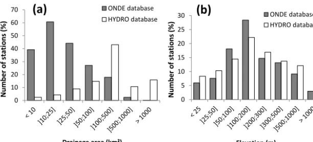
Figure 2 illustrates the complementary nature of the ONDE network to the already existing HYDRO (http://www. hydro.eaufrance.fr, last access: 22 May 2018) French river flow monitoring network. The ONDE sites and a set of 1600 gauging stations available in the HYDRO database have been projected on the RHT (Theoretical Hydrographic Network; Pella et al., 2012) river network and the drainage area and the elevation have been estimated. A large part of ONDE sites are located on small headwater streams, with 70 % of the sites with a drainage area of less than 50 km2, while most of the gauging stations record flows of catchments of medium size (between 100 and 500 km2). Only four stations display a drainage area of more than 1000 km2. The distributions of elevation of the two databases look similar. The ONDE sites are mostly located on rivers with an elevation below 200 m (75 % of sites). The ONDE sites are sparse at high elevations (95 sites located above 1000 m). This bias is likely due to access difficulties in mountainous areas.

2.3 POC dataset: a denser regional dataset used for independent validation

be-0 10 20 30 40 50 60 70 ((

N

u

mbe

r

o

f s

ta

ti

o

n

s

(%)

Drainage area (km²) ONDE database HYDRO database

0 5 10 15 20 25 30

N

u

mbe

r

o

f s

ta

ti

o

n

s

(%)

Elevation (m)

ONDE database HYDRO database

(a)

(b)

Figure 2.Distribution of the 3300 ONDE sites and of the 1600 gauging stations available in the HYDRO database against(a)drainage area and(b)elevation.

tween June and October, resulting in eight observations per year. Four intermittency statuses were available in the POC dataset (Datry et al., 2016a), but to allow comparisons with the ONDE network, we pooled the two “Flowing” and “Low Flow” POC statuses into a single “Flowing” status and the two “No flow” and “Dry” statuses into the “Drying” status. This dataset is available as maps with flow states assigned to the inspected streams. Values of RPoD at each POC ob-servation date are calculated in the same way as RPoDONDE.

Thus RPoDPOCis given by the ratio between the number of

drying statuses and the total number of observations at each inspected stream located in the same HER2–HR.

2.4 Explanatory discharge dataset

Two discharge datasets (continuous daily time series) were used as explanatory variables of discrete intermittence ob-servations, with the objective of extrapolating the intermit-tence frequency over time. The two datasets included time series of daily discharge extracted from the French river flow monitoring network (HYDRO database, http://www.hydro. eaufrance.fr/, last access: 22 May 2018): (i) the 2011–2017 dataset with full records available between 1 January 2011 and 31 June 2017; (ii) the 1989–2017 dataset concerning a reduced number of gauging stations and providing daily discharges between 1 January 1989 and 31 June 2017. Ac-cording to the hydrometric services in charge of the selected gauging stations, high quality of measurements was ensured and observed discharges were not or only slightly altered by human actions.

The 2011–2017 dataset was composed of 1600 gauging stations distributed across France. Each stream where a HY-DRO gauging station is located has been defined as IRES or perennial. Several definitions of IRES can be found in the literature (Huxter and van Meerveld, 2012; Eng et al., 2016; Reynolds et al., 2015). In this study, we considered stations to be intermittent when five consecutive days with discharge

less than 1 L s−1 have been observed during the period of record.

The 1989–2017 dataset consisted of 630 gauging stations selected with less than 5 % of missing data (continuous or not) during the period 1989–2017. This dataset was there-after used to estimate the regional probability of drying be-fore the creation of the ONDE network.

2.5 Explanatory groundwater-level dataset

50

1

0.1

0.01

1 0.8 0.6 0.4 0.2 0

166

165

164

1 0.8 0.6 0.4 0.2 0 Non-exceedance frequency

of groundwater level Non-exceedance frequency

of discharge

3. Average of non-exceedance frequency (F) of observed discharge and groundwater level between observa�on date d and d-5

0 10 20 30 40 50 60

0 0.2 0.4 0.6 0.8 1

RP

oD

(%)

Average of non-exceedance frequency (F) RPoDLLR= -27.4 x ln(F) - 12.8

R² = 0.85

0 10 20 30 40

15/5/12 9/7/12 2/9/12 27/10/12

RP

oD (%)

RPoDLLR

1. Selec�on of ONDE sites, gauging sta�ons and piezometers by HER2-HR combina�on

HR4 HR6 HR1

4. Fi�ed analy�cal formulas 5. Predicprobability of drying (RPoD)�on of daily regional 2. Regional probability

of drying at ONDE sites RPoDONDE ONDE site Gauging station (Q) Piezometer (GW)

RPoDLR RPoDLR = exp (0.6 - 7.4F)

1 + exp (0.6 - 7.4F) R² = 0.9 Observa�ons HER2 n°97

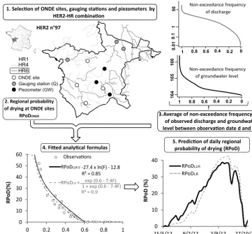
Figure 3.Strategy of parametric modelling (steps 1–4) developed to predict (step 5) the regional probability of drying (RPoD) by HER2–HR combination in France.

2.6 Statistical modelling of regional probability of drying

The parametric modelling strategy was based on five main steps (Fig. 3). The first step consisted in selecting all ONDE sites, gauging stations and piezometers located in the same HER2–HR combination. When the total number of gauging stations and piezometers was less than five for a HER2–HR combination, we merged the HER2–HR combination with a neighbouring one located in the same HER1. This was done for 20 of the 280 regions. The second step consisted in cal-culating the RPoDONDEfor each observation date (5 year−1)

and for all selected ONDE sites. In a third step, a flow dura-tion curve was determined for each selected HYDRO gaug-ing station. The average non-exceedance frequency of the observed discharge at gauging stations was averaged for the date of observation (d) at ONDE sites and the 5 days pre-ceding the observation. The lag of 6 days accounted for the fact that ONDE survey dates in a region could differ by 5 days, and accounted for the inertia of physical processes (e.g. storage capacity). The same operation was carried out

with selected piezometers. Finally the hydrological condi-tions are described by the average (across stacondi-tions)F of the non-exceedance frequencies of discharge (Fq) and

ground-water levels (Fgw) with respect to the relative proportions of gauging stations and piezometers:

F (d)=

i=Nq

P

i=1

Fqi+

j=Ngw

P

j=1

Fgwj

(Nq +Ngw)

, (2)

whereFqi denotes the average non-exceedance frequency of

discharge at the gauging stationicalculated betweend and

d−5;Fgwjthe average non-exceedance frequency of

ground-water levels at the piezometerj calculated betweend and

d−5;Nqthe number of gauging stations selected in a HER2–

HR combination; and Ngw the number of selected piezome-ters selected in the HER2–HR combination. The fourth step consisted in estimating the RPoDONDE as a function of F.

– A truncated logarithmic linear regression (LLR), with two parametersα1andβ1:

RPoDLLR(d)=

min(1;α1×ln(F (d))+β1)whenF < F0

0 whenF ≥F0. (3)

F0 was fixed as the value of non-exceedance frequen-cies of discharge and groundwater levels at which no more drying status was observed across the ONDE net-work (RPoDONDE=0).

– A logistic regression (LR) with two parametersα2and

β2:

Logit(RPoDLR(d))=ln

_RPoD

LR(d)

1−RPoDLR(d)

=α2×F (d)+β2. (4)

LR is a multivariate analysis method well known for its relevance in binary classification issues (Lee, 2005). The RPoDLRwas then calculated as follows in Eq. (5):

RPoDLR(d)=

exp(α2F (d)+β2)

1+exp(α2F (d)+β2). (5)

Models were calibrated against observations available during the same period, 2012–2016, leaving out the year 2017 for an independent validation test. However, for the continuous temporal extrapolations (one over 2011–2017, the other over 1989–2017), two models were built with different piezometers and gauging sta-tions selected as explanatory variables (see Sects. 2.4 and 2.5). Thus there are two sets of regression param-eters specific to each dataset for both the LLR and LR models, leading to different prediction of RPoD. Finally, in a fifth step, a daily regional probability of dry-ing (RPoD) could be predicted for each HER2–HR combina-tion with both models following analytical formulas (Eqs. 3 and 5).

2.7 Model robustness: validation using independent datasets

We used (1) the POC independent data and (2) the 2017 ONDE year to test the robustness of the LLR and LR model to predict the intermittence frequency (1) in space and (2) over time. Note that when predicting on the POC datasets, a new model was calibrated using only ONDE sites located out of POC streams.

For both datasets (POC and ONDE, 2017), the relative performance of the LLR and LR models was compared in multiple ways using both the 2011–2017 and 1989–2017 datasets. The performance of each model was evaluated by

the Nash–Sutcliffe efficiency criterion (NSE) (Nash and Sut-cliffe, 1970):

NSE=1−

N P

i=1

(RPoDONDEi−RPoDpri)2

N P

i=1

(RPoDONDEi−RPoDONDEi)2

, (6)

where RPoDONDEi is the average proportion of drying

sta-tuses over the ONDE sites located in the HER2–HR combi-nation at theith observation date, RPoDpriis the predicted

regional probability of drying at the ith observation date,

RPoDONDEiis the mean of RPoDONDEiover the period and

Nis the total number of observations in the ONDE network for each HER2–HR combination.

2.8 Model prediction

Both models have been calibrated over the period 2012–2016 and were then applied in a fifth step to predict the daily RPoD in France (Fig. 3). The RPoD was firstly predicted over the period 2012–2016 in order to identify the most affected re-gions by flow intermittence using the 2011–2017 datasets. The second application concerned the extrapolation of RPoD in France over a longer period using the 1989–2017 dataset to analyse the temporal variability of flow intermittence at the national level. It should be noted that model predictions only concern streams with a Strahler order of lower than 5 due to the ONDE site location.

3 Results

3.1 Quantitative analysis

3.1.1 Inter-annual intermittence according to the raw discrete ONDE network

A total of 1127 ONDE sites have recorded at least one drying event during the period 2012–2016 representing 35 % of the 3300 ONDE sites. From the ONDE database the probabil-ity of drying at the country scale was computed as the total number of drying statuses over France divided by the total number of ONDE observations available during statuses the same year (Fig. 4a). Between 2012 and 2016, the most crit-ical year is 2012, with 15 % of drying statuses followed by 2016 (14 %) and 2015 (14 %) (Fig. 4a). The years 2013 and 2014 are less affected with only 6 % of drying statuses ob-served (Fig. 4a).

(18161) (17086) (17269) (20577) (17990)

0 10 20 30

May Jun Jul Aug Sep

2012 2013 2014 2015 2016

85 93 93 86 86

15 7 7 14 14

0 20 40 60 80 100

2012 2013 2014 2015 2016

Pr

opor

�

on of dr

ying

(%)

Drying Flowing

Pr

opor

�

on of dr

ying

(%)

(a) (b)

Figure 4. (a) Distribution of the yearly proportion of drying observed with the ONDE network with the total yearly number of ONDE observations written in brackets and(b)distribution of proportions of drying per year and per month.

lower than in 2012, but follows the same pattern with an in-crease at the end of July (3 %), reaching 9 % in August and in September. In 2014, the first peak of drying (5 %) is reached early in June. Then, the proportion of drying decreases in July (3 %) and increases slightly in August (4 %), reaching 7 % in September. In 2015, the critical period occurs at the end of July with 19 % of drying statuses, and the proportion of drying decreases slightly at the end of August (17 %) until it reaches 9 % in September. Finally, in 2016, the situation gradually deteriorates every month, reaching 20 % of drying statuses in August, and 28 % in September.

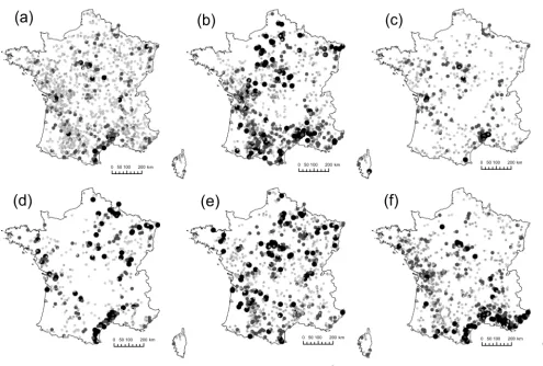
Between 2012 and 2016, a proportion of drying higher than 50 % is recorded on 93 ONDE sites and their spatial distribution is very patchy at the scale of France (black and dark grey dots, Fig. 5a). There are only 158 ONDE sites with at least one drying event every year and a variability of drying locations can be observed across years. The south-east of France is heavily affected by rivers drying, where the proportion of drying can exceed 75 % annually (black dots, Fig. 5b–f). The north-western part of France is less affected, although many ONDE sites show a proportion of drying ob-served above 50 % in 2014 and 2016 (Fig. 5d and f). North-eastern France is rather affected in 2012, 2014 and 2015, where several ONDE sites have more than 75 % of drying statuses (Fig. 5b, d and e). South-western France is particu-larly affected in 2012 and 2015 (Fig. 5b and e).

3.1.2 Comparison of flow intermittence between the raw ONDE and HYDRO datasets

The HYDRO dataset includes 90 gauging stations located on streams considered IRES, which represents only 5.6 % of the 1600 gauging stations against 35 % for ONDE sites. At the national scale, the number of IRES seems underrepre-sented in the south-western, central, and north-eastern parts of France and Corsica in comparison with sites experiencing drying in the ONDE network (Fig. 6).

Table 1.Annual statistics on flow intermittence calculated on HY-DRO gauging stations between 1 May and 30 September.

Stations with Stations with Frequency of at least one drying > 50 % discharge < 1 L s−1 drying event

2012 79 19 32.7

2013 47 14 37.9

2014 54 15 32.9

2015 76 21 31.1

2016 71 19 28.6

The number of gauging stations with at least one dry-ing event (discharge < 1 L s−1) observed between May and September varies between 79 in 2012 and 47 in 2014 (Ta-ble 1). The lowest numbers of gauging stations with dry-ing events are observed in the years 2013 and 2014, while the highest numbers are related to the years 2012, 2015 and 2016. This finding is consistent with the analysis of the ONDE network (Fig. 5a, d). The frequency of drying, corre-sponding to the ratio between the number of dry days and the total number of days between 1 May and 30 Septem-ber (153 days), in contrast, is quite constant over the years (∼30 %). The number of gauging stations with drying events over more than 50 % of the time varies little between wet years (14 in 2013) and dry years (21 in 2015), unlike ONDE observations, suggesting a significant temporal variability in the frequency of drying between dry and wet years (Fig. 5). 3.2 Validation of the predicted regional probability of

drying

3.2.1 Regression results

0 050100 200Km

0 50100 200km 050100 200km

0 50100 200km 050100 200km

050100 200km

!

( 0 –25 % !(25 % – 50 % !(50 – 75 %

!

(

(b)

(c)

(d)

(e)

(f)

(a)

km 050100 200km

Figure 5.Distribution of the percentages of drying observed at ONDE sites for the years(a)2012–2016,(b)2012,(c)2013,(d)2014,

(e)2015 and(f)2016.

! ! ! ! ! ! !!!! ! ! !!! ! !!!! !!! ! ! !!!! ! ! ! ! ! ! ! ! !! ! ! ! ! ! ! ! ! ! ! !!!! ! ! !! ! ! ! ! !!! ! ! ! ! !! ! ! ! ! !! ! !! ! ! ! ! ! ! !!! ! ! ! !! ! ! ! ! ! ! ! ! ! !! ! !! ! ! ! ! ! ! ! ! ! ! !! ! ! ! ! ! ! ! ! ! ! ! ! ! ! ! ! ! ! !! ! ! !! ! ! ! ! ! !! ! ! ! ! ! !!! ! ! ! ! ! ! ! !!! !! ! ! ! ! !! ! ! ! ! ! ! ! ! ! ! ! ! !! ! ! ! ! ! !! ! ! ! ! ! ! ! !! ! ! ! ! !! ! ! !! ! ! ! ! ! ! ! ! ! ! ! ! ! ! ! ! ! ! ! ! ! ! ! ! ! ! !!! ! ! ! ! ! ! ! ! ! !! !! ! ! !! !!!! ! ! ! ! ! ! ! ! ! ! ! ! ! ! ! ! ! ! ! ! ! ! ! !! ! ! ! !!! !! ! ! ! ! ! !! ! ! ! ! ! !! ! ! ! ! ! !! ! ! ! ! ! !!! ! ! !!!!! ! ! ! ! ! !! !!! !! ! ! ! ! ! ! ! ! ! ! !! ! ! !! ! ! ! ! ! ! ! ! ! ! ! ! ! ! ! !! ! !! !! ! ! !! !!! ! !! ! !! ! ! !! ! ! ! ! ! ! ! ! ! ! ! ! !!!! ! ! ! ! !! ! ! ! !! ! ! ! !! ! ! ! ! ! ! ! ! ! ! ! ! ! ! ! !! !!!!! ! !! ! ! ! ! !!!!!!!!!!! ! ! ! ! !! !! !! ! ! ! ! ! ! ! ! !! ! ! ! ! ! ! ! !! ! ! ! ! ! !! ! ! ! ! ! ! ! !! ! !!! ! ! !!!! ! !!!! !! ! ! ! ! ! ! !!! ! ! ! !!! !!! ! ! ! ! !! !! !! ! ! ! ! !!! ! !! ! ! !! !!!!!! ! !! ! ! !! !!!!!!! !! !! !!!! !!!! !! ! !!!! ! ! ! ! ! ! ! ! ! ! !! ! ! ! ! ! ! ! ! ! ! ! ! ! !! ! ! ! ! ! ! ! ! ! ! ! ! ! ! ! ! ! ! ! !!!!! ! ! ! ! ! ! ! ! ! ! ! ! ! ! ! ! ! ! ! ! ! ! ! ! !! ! ! ! ! ! ! ! ! ! ! ! ! !!!! ! ! ! ! ! ! ! ! ! ! ! ! ! ! ! !! ! ! ! ! ! ! ! ! ! ! ! ! ! !! !! ! ! ! ! ! !! !_{! !}!!! ! !! !! ! ! !! ! ! ! !!!!!!!!!! ! ! ! ! !!! ! !!! ! ! ! ! ! !!! !!! !!!!!!! ! !!!!!!!!! ! ! ! ! !! ! ! ! ! ! ! ! !! ! ! ! ! !!!! ! ! !! ! ! !! !! !!! ! ! ! ! ! ! ! ! ! ! ! ! ! ! ! !! ! ! ! ! !! ! ! ! !! ! ! ! ! ! !!! ! ! !! ! ! ! !!! ! !!! ! ! ! !! !!! ! !!! ! ! ! ! ! !! !! ! ! ! ! ! ! ! ! ! ! ! ! !! ! !! ! ! ! ! ! ! ! ! ! ! ! !! ! ! ! ! ! ! !!!! ! ! ! !! ! !! ! ! ! ! !! ! ! ! ! ! ! ! ! ! !! ! !! !! !! ! ! ! ! !!! ! ! ! !!! ! ! !! ! ! ! ! ! ! !! ! ! ! ! ! ! ! ! ! ! ! ! ! ! ! ! ! ! ! ! ! ! ! ! ! ! ! ! ! ! ! ! ! !! ! ! !!!!! ! ! ! ! ! !! ! ! ! ! ! !! ! ! !!! ! ! ! ! ! ! ! ! ! ! ! ! ! ! ! ! ! ! ! ! ! ! ! ! !! ! ! ! ! ! ! ! ! !! ! ! ! !! ! ! ! ! ! ! !! ! ! ! !!! !!!!!!!!!!!! ! ! ! ! ! ! !!!!! !! ! ! ! !!!! ! ! !! ! ! ! ! ! ! ! ! ! ! ! ! ! ! ! ! ! ! ! ! !! ! ! ! ! ! ! ! !!! ! ! ! !! ! ! !! !! ! ! ! ! ! ! ! ! ! ! ! !! ! ! ! ! ! !! ! ! ! !! ! !! ! ! !! ! ! ! ! ! ! !! ! ! ! ! ! ! ! ! !!! ! ! ! ! ! ! ! ! ! ! ! !! ! ! ! ! ! ! ! !! ! ! !! !!!! !! ! ! !! ! !!! !! ! ! ! !!! ! !! !_{! !} ! ! ! ! ! ! ! ! ! !!!!!!!!!!!! ! ! ! ! ! ! ! ! !! ! !!!!!! ! ! ! ! ! ! !!!!!!!! ! ! ! ! !!!!! !!! !!!!!! ! ! ! ! ! !!! !!!!!!!!!! ! ! ! ! ! ! !! ! ! ! ! ! ! ! ! !! ! ! ! ! ! ! ! ! ! ! ! ! ! ! ! ! ! ! ! ! ! ! !!!! !!! !! !!! ! !! ! ! !!!! ! !!! ! ! ! ! ! ! ! ! !!!!!! ! ! ! ! ! ! !!!!!!! !! !! ! ! ! ! !!!! !! !! ! ! !!!!!! ! ! ! !! ! ! ! ! !! !! ! !!!!! !!! ! !! ! ! ! ! !!! ! ! ! ! ! !!! !!!!! ! ! ! !!! ! ! !! !! !! ! ! ! !! !! !!!!!! ! ! !!!! ! ! ! !! ! ! ! ! ! ! ! ! ! ! ! ! ! ! ! ! ! ! ! ! ! ! ! ! !! ! ! ! ! ! ! ! ! ! ! ! ! ! ! ! ! ! ! ! ! ! !! !! ! !! ! ! ! ! ! ! ! ! ! ! ! ! ! !! ! ! ! ! ! ! ! !! !! ! !! ! !! !! ! ! ! ! ! !! !!!!_! !!!

! Intermittent gauging station HYDRO

! _{ONDE site with no-flow}

0 50100 200km

±

Figure 6.Map of ONDE sites and HYDRO gauging stations with at least one drying.

model (Fig. 7a and b). With the LR model, 50 % of the HER2–HR combinations obtain a NSE greater than 0.8, rep-resenting a coverage of 65 % of the French territory, while 33 % of HER2–HR combinations display a NSE higher than 0.8 (50 % of coverage of France) with the LLR model. Re-gions with the highest performances are located in sedimen-tary plains, in the south-east of France and in the Pyrenees Mountains. Conversely, the worst performances are obtained in the mountainous regions of the Alps as well as in the Massif Central. In these regions the size of the HER2 is rather small and the number of ONDE sites, gauging stations and piezometers per HER2–HR combination are certainly too few to derive reliable relations. Despite pooling, estimat-ing RPoD remains impossible for nine HER2–HR combina-tions (4.5 % of coverage of France) because the number of ONDE sites, gauging stations and piezometer sites is insuffi-cient (less than five) to perform the regression analysis.

Figure 7.Map of Nash–Sutcliffe criteria (NSE) obtained for each HER2–HR combination between 2012 and 2016 with the 2011–2017 and 1989–2017 datasets according to(a)and(c)a log-linear regression (LLR) model; or(b)and(d)a logistic regression (LR) model. NSE differences between the 2011–2017 dataset and the 1989–2017 dataset are represented for(e)the LLR model and(f)the LR model.

The LR and LLR models lead to a similar performance range. However, the LR model outperforms the LLR model in terms of number of HER2–HR combinations, with NSE greater than 0.8 (Fig. 7c and d). The performance is sensitive

with the most degraded values of NSE are small HER2–HR combinations located in eastern France (Fig. 7e and f).

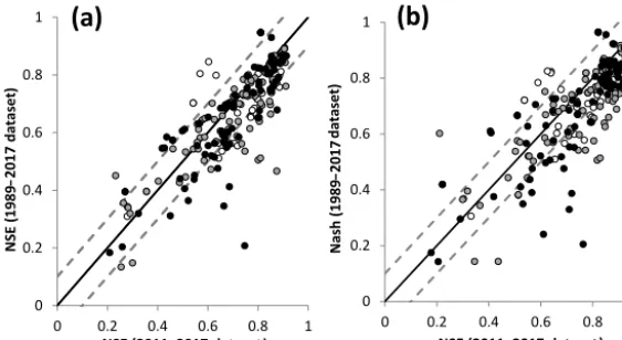
The decrease in performance is mainly due to the differ-ence in the number of gauging stations and piezometers be-tween the two datasets (Fig. 8). The most degraded NSEs correspond to HER2–HR combinations where the number of gauging stations and piezometers considered in regressions is the most reduced, i.e. with a loss higher than 50 % of the stations (black and dark grey dots; Fig. 8a and b). However, the decrease in performance remains low (the difference in NSE is below 0.1 for 75 and 64 % of HER2–HR combina-tions with the LLR and LR models, respectively).

3.2.2 Comparison to the POC database

The observed proportion of drying RPoDPOCis rather well

simulated by both LLR and LR models with the 2011–2017 explanatory dataset (NSE > 0.7 except for the year 2011; Fig. 9). In addition, the models are able to capture small fluctuations of RPoDPOC during the summer period. The

best results during the year 2011 are obtained with the LLR model (black curve; Fig. 9) and the LR model overestimates RPoDPOC by 3 % (dashed grey curve; Fig. 9). In 2012, the

decline in water levels is more gradual than in 2011 and a marked peak is reached in September with 40 % of RPoDPOC

(Fig. 9). This pattern is well reproduced by both models with a good fit to all observation points (Fig. 9). The year 2013 is less affected by drying occurrence and the maxi-mum RPoDPOC does not exceed 20 % (Fig. 9). Curves of

both models fit to observations well until the end of August. Note that the LR model is slightly closer to the observations around the peak in September compared to the LLR model. However, the LR model overestimates the RPoDPOC at the

end of September and in October.

When the 1989–2017 dataset is used for explanatory vari-ables, the simulations of RPoD are weakly degraded with both models (Fig. 9d, e, f). However, the simulated pattern is similar to the observed one. The LLR model outperforms the LR model during the 3 years of validation with the 1989– 2017 dataset (black curve; Fig. 9d, e, f).

3.2.3 Temporal patterns assessment of models between 2012 and 2017

During the calibration period, the LLR and LR models tend to better simulate the RPoD during dry years 2012 and 2016 (NSE=0.8 with the LLR and LR models; Table 2) than during wet years (e.g. 2014 with NSE < 0.7). The NSEs are lower during the months of May and June when few drying events are observed, while NSEs are much better during the driest months of August and September.

During the validation year of 2017, both models obtain a similar performance over the year independent of datasets (NSE=0.7).

Monthly NSEs in 2017 follow the same trend as monthly NSEs of the calibration period, with lower NSEs in May (NSEs < 0.4) and June (NSEs=0.5) and higher NSEs in July, August and September (NSEs=0.6) with both models inde-pendent of datasets. Figure 10 shows the dispersion between predicted RPoD and drying statuses observed at ONDE sites in the scatter plot during the validation year 2017 (Fig. 10a and b) in comparison with the year 2012, which obtains the better NSE during calibration period (Fig. 10c and d). The NSEs obtained in 2017 are 0.72 with the LLR model and 0.68 with the LR model against 0.83 and 0.81 in 2012, spectively. The performance is slightly lower in 2017 but re-mains acceptable with NSEs close to 0.7, and both models seem able to predict RPoD from the calibration period. 3.3 Application of regional models

3.3.1 Modelling of intermittencies severity between 2012 and 2016

Both models have been applied using the 2011–2017 dataset. Figure 11 displays the maximum number of consecutive days (DRPoD>20 %) with RPoD higher than 20 % simulated by

both the LLR and LR models. The most affected regions are located in the south-east of France and in the sedi-mentary plains, which is consistent with the spatial pattern obtained from the ONDE observations (Fig. 5). The most impacted year followed the same hierarchy: the year 2012 is the most critical year, with 30 % of France displaying DRPoD>20 %higher than 60 days followed by the year 2015

(20 % of France with DRPoD>20 %> 60 days) and 2016 (15 %

of France with DRPoD>20 %> 60 days) (Fig. 11). The years

2013 and 2014 are weakly affected, with 5 % and 6 % of France with DRPoD>20 %higher than 60 days, respectively.

The LR model tends to simulate shorter periods of drying, particularly in HER2–HR combinations located in south-eastern France in 2013 and 2014 (Fig. 11). However, there is an overall agreement between RPoD simulated by both mod-els in terms of spatial and temporal extent of dry streams. 3.3.2 Reconstitution of historical regional probability

of drying

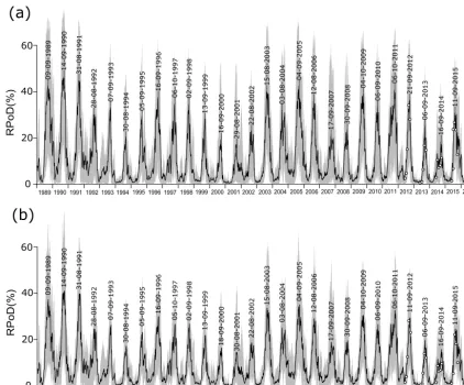
The trend temporal patterns of RPoD predicted by the two models, considering the 1989–2017 dataset, look similar be-tween 1989 and 2016, and the simulated RPoD fit well to RPoDONDE(Fig. 12).

0 0.2 0.4 0.6 0.8 1

0 0.2 0.4 0.6 0.8 1

N

SE

(

1

9

8

9

–

NSE (2011–2017 dataset

0 0.2 0.4 0.6 0.8 1

0 0.2 0.4 0.6 0.8 1

N

as

h

(

1

9

8

9

–2

0

1

7

NSE (2011–2017 dataset

(b)

(a)

2

0

1

7

d

at

as

e

t)

d

at

as

e

t)

) )

Figure 8. NSE calculated for each HER2–HR combination between 2012 and 2016 with the 1989–2017 dataset as a function of NSE calculated with the 2011–2017 dataset with, respectively,(a)the LLR model and(b)the LR model. The colours of the dots represent the proportion of gauging stations and piezometers lost between the 2011–2017 database and the 1989–2017 database: losses < 50 % (white); losses between 50 and 75 % (grey); losses > 75 % (black).

The highest values of RPoDs (above 35 % over France) are observed in 1989, 1990, 1991, 2003 and 2005 (black curve, Fig. 12a and b). The RPoDs simulated during these dry years are out of the range of the observed values over the cali-bration period (2012–2016). Estimations are thus uncertain. However, the high values of RPoD are consistent with ob-servations reported in previous studies (e.g. Larue and Giret, 2004; Snelder et al., 2013; Caillouet et al., 2017). Conversely, the years less affected by drying are simulated in 1994, 2001 and 2014, with an average RPoD below 15 % throughout the year (black curve, Fig. 12a and b).

Results obtained with the LLR model are more contrasted in terms of extreme values than those obtained with the LR model (Fig. 12b).

4 Discussion

4.1 ONDE network complementarity with conventional flow monitoring network

The analysis of the ONDE observations shows that the pro-portion of rivers undergoing drying is significantly higher (35 %) than that observed with the conventional monitor-ing (HYDRO database, 8 %). This proportion, although re-lated to a short period of records 2012 and 2016, is consis-tent with the percentage of 39 % of river segments classi-fied as intermittent by Snelder et al. (2013). This analysis confirms the under-representation of IRES in the French HY-DRO database, and probably others in other countries (flows are often uncontrolled in IRES). Without gauging stations lo-cated on headwaters, Snelder et al. (2013) were unable to predict IRES in eastern France (see Fig. 9, p. 2694). The high density of ONDE sites makes it possible to improve the detection of drying events and lead to better understand

the spatial distribution of IRES located at the upstream ex-tent of the hydrographic network. The ONDE network en-compasses various hydrological conditions, which provides a more accurate assessment of inter-annual variability, dif-ferentiating between dry years (2012, 2015 and 2016) and wet years (2013, 2014) with clearly few drying occurrences. The validation of the LR and LLR models against the spa-tially dense POC database also demonstrates the spatial rep-resentativeness of the ONDE network. Thanks to the qual-itative information provided and to models such as the sta-tistical models developed here, it is now possible to capture drying events at the regional scale.

The ONDE sites are located on small headwater streams which can be very reactive to external disturbances (rainfall deficit, change in air temperature, increase in water with-drawals, etc.) and by nature are more likely to be IRES. The gauging stations available in the HYDRO database are located on larger streams and their hydrologic response to changes in external factors (environmental or human) is slower and drying occurred with greater inertia under tem-perate climate. Their uneven distribution across France does not allow us to accurately characterise the inter-annual vari-ability of drying development. Overall, the ONDE network provides very complementary information to conventional flow monitoring, leading to a better understanding of the pro-cesses of drying in upstream catchments.

0 5 10 15 20 25 30 35 40 45

01/04/2011 30/06/2011 28/09/2011 27/12/2011

RP

oD (%)

0 5 10 15 20 25 30 35 40 45

15/05/2012 09/07/2012 02/09/2012 27/10/2012

0 10 20 30 40

15/05/2013 13/08/2013 11/11/2013 0

10 20 30 40

15/05/2012 13/08/2012 11/11/2012 0 5 10 15 20 25 30 35 40 45

15/05/2013 13/08/2013 11/11/2013

0 10 20 30 40

17/04/2011 16/07/2011 14/10/2011

RPoD simulated with the 1989–2017 dataset: RPoD simulated with the 2011–2017 dataset:

NSE LLR = 0.92 NSE LR = 0.75

NSE LLR = 0.88 NSE LR = 0.94

NSE LLR = 0.89 NSE LR = 0.92

NSE LLR = 0.86 NSE LR = 0.85

NSE LLR = 0.88 NSE LR = 0.87 NSE LLR = 0.89

NSE LR = 0.69

LLR model LR model Obs - POC data

RP

oD (%)

(a)

(d)

(b)

(e)

(c)

(f)

Figure 9.Comparison between observed proportion of drying RPoDPOCand RPoD predicted by the LLR and LR models with the 2011–2017

dataset in(a)2011,(b)2012 and(c)2013 and with the 1989–2017 dataset in(d)2011,(e)2012 and(f)2013.

Table 2.NSE criteria obtained between 2012 and 2017 with the LLR and LR models calibrated over the period 2012–2016.

2011–2017 dataset 1989–2017 dataset

Calibration Valid. Calibration Valid.

2012 2013 2014 2015 2016 2017 2012 2013 2014 2015 2016 2017

LLR model

May 0.2 0.0 0.5 0.5 0.6 0.4 0.2 0.0 0.3 0.0 0.7 0.2

Jun 0.6 0.3 0.8 0.5 0.8 0.5 0.6 0.3 0.5 0.3 0.8 0.5

Jul 0.7 0.5 0.6 0.6 0.8 0.7 0.7 0.5 0.5 0.4 0.8 0.6

Aug 0.8 0.6 0.7 0.7 0.8 0.6 0.7 0.5 0.5 0.5 0.8 0.6

Sep 0.7 0.8 0.6 0.6 0.7 0.6 0.6 0.7 0.5 0.5 0.6 0.6

May–Sep 0.8 0.8 0.7 0.7 0.8 0.7 0.8 0.7 0.5 0.6 0.8 0.7

LR model

May 0.2 0.0 0.5 0.1 0.6 0.3 0.3 0.0 0.3 0.0 0.7 0.2

Jun 0.6 0.5 0.8 0.5 0.8 0.4 0.6 0.4 0.5 0.3 0.7 0.4

Jul 0.7 0.6 0.5 0.6 0.8 0.6 0.7 0.4 0.5 0.4 0.8 0.6

Aug 0.7 0.6 0.7 0.6 0.7 0.6 0.6 0.4 0.5 0.4 0.7 0.5

Sep 0.6 0.8 0.6 0.7 0.7 0.6 0.5 0.6 0.4 0.5 0.6 0.6

0 10 20 30 40 50 60 70

0 10 20 30 40 50 60 70

%NoFo

b

s

2

0

1

7

%NoFL 2017

0 10 20 30 40 50 60 70

0 10 20 30 40 50 60 70

%NoFo

b

s

2

0

1

7

%NoFL 2017

NSE = 0.7

0 10 20 30 40 50 60 70

0 10 20 30 40 50 60 70

%NoFo

b

s

2

0

1

2

%NoFL 2012

0 10 20 30 40 50 60 70

0 10 20 30 40 50 60 70

%NoFo

b

s

2

0

1

2

%NoFL 2012

NSE = 0.7

NSE = 0.8 NSE = 0.8

(a)

(b)

(c)

(d)

Figure 10.Scatter plot of the predicted RPoD (xaxis) and drying observed at ONDE sites (yaxis) in 2017 and 2012 simulated with the 2011–2017 dataset by (aandc) the LLR model and (bandd) the LR model.

DRPoD>20 % of LLR simulations

DRPoD>20 % of LR simulations

> 90 days 60–90 days

30–60 days 1–30 days

0 days

1 1

2012

2012

2013

2013

2014 2015 2016

2015

2014 2016

Figure 11.Maximum duration of consecutive days with RPoD higher than 20 % simulated with the LLR and LR models.

datasets. The accuracy of the predictions is dependent on the number of gauging stations, ONDE sites and piezome-ters available to calibrate the regressions. The highest NSEs are obtained in western sedimentary plains and south-eastern

RPoD(

%)

198919901991199219931994199519961997199819992000200120022003 200420052006200720082009 20102011 20122013201420152016

40

20

0 ●

● ● ● ●

●● ● ● ●

● ● ●●

● ● ● ●

● ●●

● ●●

RPoD(

%)

198919901991199219931994199519961997199819992000200120022003 200420052006200720082009 20102011 20122013201420152016

60

40

20

0 ●

● ● ● ●

●● ● ● ●

● ● ●●

● ●

● ● ● ●

●● ● ●●

(a)

(b)

● ●

●● ● ● ●

● ● ●●

●

● ●● ●

● ● ● ●

●

● ●●

●

●● ● ●

●

●● ● ●_●

● ● ●●

●

● ● ● ●

●

●● ● ●●

09-198

9

14-

09-199

0

31-

08-199

1

28-

08-199

2

07-

09-199

3

30-

08-199

4

05-

09-199

5

16-

09-199

6

06-

10-199

7

02-

09-199

8

13-

09-199

9

16-

09-200

0

29-

08-200

1

22-

08-200

2

15-

08-200

3

03-

08-200

4

04-

09-200

5

12-

08-200

6

17-

09-200

7

30-

09-200

8

04-

10-200

9

06-

09-201

0

06-

10-201

1

21-

09-201

2

06-

09-201

3

16-

09-201

4

11-

09-201

5

13-

09-201

6

60

09-198

9

14-

09-199

0

31-

08-199

1

28-

08-199

2

07-

09-199

3

30-

08-199

4

05-

09-199

5

16-

09-199

6

05-

10-199

7

02-

09-199

8

13-

09-199

9

18-

09-200

0

30-

08-200

1

22-

08-200

2 _15-

08-200

3

03-

08-200

4

04-

09-200

5

12-

08-200

6

17-

09-200

7

30-

09-200

8

04-

10-200

9

06-

09-201

0

06-

10-201

1

11-

09-201

2

06-

09-201

3

16-

09-201

4

11-

09-201

5

13-

09-201

6

Figure 12.RPoD simulated between 1989 and 2016 with the 1989–2017 dataset with(a)the LR model and(b)the LLR model. The grey area represents the RPoD between the 90th percentile and the 10th percentile simulated on the HER2–HR combination, the black curve represents the average RPoD simulated by the HER2–HR combination and white dots represent the mean RPoD_ONDEfor each observation date. Dates mentioned correspond to the day of the maximum average RPoD simulated by the HER2–HR combination (black curve) of each year.

which corresponds to the monitoring period of the ONDE database. They benefit from a dense monitoring network (gauging stations, ONDE sites, piezometers), which allows a better representation of the hydrological functioning of streams located within the same HER2. Conversely, perfor-mance was poor in mountainous areas such as in the Alps or the Massif Central (NSE < 0.4) where river flow regimes are diversified combining rainfall and snowmelt influences. By construction, the area of HER2–HR combination in moun-tains is reduced, which leads to a limited number of monitor-ing stations, certainly not sufficient to fit the models. More-over, the observation period for ONDE sites was limited be-tween May and September and dryings can be missed, par-ticularly for streams influenced by snow or ice melting with potential drying periods in winter. In regions potentially con-cerned with drying events from the May–September period, the actual ONDE monitoring strategy needs to be adapted to

provide reliable temporal observations and extrapolations of drying frequencies.

0 0.2 0.4 0.6 0.8 1

0 0.2 0.4 0.6 0.8 1

0 0.2 0.4 0.6 0.8 1

0 0.2 0.4 0.6 0.8 1

NSE with discharge and groundwater level NSE with discharge and groundwater level

NSE with di

schar

ge only

NSE with di

schar

ge only

(b)

(a)

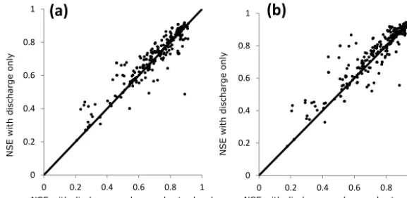
Figure 13.Comparison of NSE obtained with regression including only the discharge variable as a function of NSE obtained with discharge and groundwater-level variables in the 2011–2017 dataset with(a)the LLR model and(b)the LR model.

of piezometers is greater than 70 % in more than 30 % of HER2–HR combinations. The presence of piezometers in-creases the density of the monitoring network in HER2–HR combinations with few available gauging stations. Thanks to groundwater-level data, RPoD can be predicted on more HER2–HR combinations.

4.3 Interest in reconstructing the dynamic regional probability of drying

Spatio-temporal simulation of the probability of drying is crucial for advancing our understanding of IRES ecology and management. Some aquatic species can persist in a dry reach for a few days, weeks or months, while some are highly sen-sitive to desiccation (Datry, 2012; Storey and Quinn, 2013; Stubbington and Datry, 2013). Estimation of the total dura-tion of days with drying at the reach scale is therefore needed to understand biological patterns in river networks (Kelso and Entrekin, 2018). To our knowledge, no study has pro-posed to reconstruct daily flow-state time series of headwater streams at the country scale such as France (> 500 000 km2) using discrete observations in time and space. In the litera-ture, studies at national scale remain focused on the detec-tion and the mapping of IRES because these rivers are his-torically poorly investigated and their proportion in existing hydrographic networks remains inaccurate or misunderstood (Nadeau and Rains, 2007; Snelder et al., 2013). Recently, several studies proposed alternative methodologies in order to estimate metrics in ungauged IRES (Gallart et al., 2016) or to predict daily streamflow in river basins experiencing flow intermittence (De Girolamo et al., 2017b), but remain applicable at the local scale.

This study provides a first regional approach to use dis-crete data obtained from regular observations. The average non-exceedance frequency is a global hydrological statistic that only captures the hydrological conditions at the regional scale in modelling the RPoD. For rainfall-driven river flow regimes, the effect of rainfall events on flow intermittence at

the HER2–HR scale is probably indirectly reflected by the daily discharge and groundwater levels used to calculate the average non-exceedance frequency. However, when more ob-servation data are available, it is likely that including more detailed descriptors of rainfall events and local geology could improve our approach. In France, based on the 2011–2017 dataset, both models suggest the highest values of RPoD along the Mediterranean coast (DRPoD>20 %> 100 days each

Figure 14.Regional probability of drying simulated withF=1 % predicted with(a)the LLR model and(b)the LR model.

4.4 Validity of historical regional probability of drying during severe low-flow period

The second application aimed at reconstructing historical RPoD over the period 1989–2016. Both models suggest the highest values of mean RPoD (> 35 %) in 1989–1991, 2003 and 2005. During these dry years, predicted values of RPoD result from extrapolation but are consistent with published studies (Mérillon and Chaperon, 1990; Moreau, 2004). For example, Mérillon (1992) estimated that for the whole of France, 11 000 km of rivers were dried at the end of the sum-mers of 1989 and 1990. Caillouet et al. (2017) found that the low-flow event observed in 1989–1990 was particularly severe in terms of duration and affected 95 % of France. Snelder et al. (2013) showed from 628 gauging stations that the years 1989–1991, 2003 and 2005 witnessed particularly high values of duration and frequency of drying events. They found that regions with the highest probability of drying were located along the Mediterranean and Atlantic coasts, which is consistent with ONDE observations and with our results.

Both models suggest the same sequence of dry and wet years. However, the application of the LLR model leads to less contrasted RPoD than the LR model (Fig. 12).

To illustrate these differences, the RPoD has been simu-lated by both models with an extremeF of 1 % (Fig. 14). The RPoDLLRis significantly higher and exceeds 80 % in 30 % of

the study area against only 5 % of the area with the RPoDLR.

On the other hand, models simulate low RPoD in HER2– HR combinations where the RPoDONDEis very low between

2012 and 2016, even whenF was 1 %, because this situation never occurred during the calibration period (Fig. 14). The logistic function of the LR model takes an S-shape which in-duced a decrease in the slope of the curve toward extreme values observed during the calibration period (2012–2016). The truncated logarithmic function of the LLR model is not bounded and RPoD can reach 100 % during extreme low-flow events by extrapolation. Since the ONDE network

mon-itoring period does not include a period with drought as se-vere as in the 1990s, it is not currently possible to assess the relative performance of the two models. Refining extrap-olated values requires additional information on headwater collected during more severe droughts than those observed during the last 5 years and then gives support to the pursuit of the ONDE network.

5 Conclusion