www.hydrol-earth-syst-sci.net/13/467/2009/ © Author(s) 2009. This work is distributed under the Creative Commons Attribution 3.0 License.
Earth System
Sciences
On the relationship between large-scale climate modes and regional
synoptic patterns that drive Victorian rainfall
D. C. Verdon-Kidd1,2and A. S. Kiem2
1Sinclair Knight Merz, Newcastle, New South Wales, Australia
2Environmental and Climate Change Research Group, School of Environmental and Life Sciences, University of Newcastle, New South Wales, Australia
Received: 28 August 2008 – Published in Hydrol. Earth Syst. Sci. Discuss.: 10 October 2008 Revised: 13 January 2009 – Accepted: 25 March 2009 – Published: 7 April 2009
Abstract. In this paper regional (synoptic) and large-scale climate drivers of rainfall are investigated for Victoria, Aus-tralia. A non-linear classification methodology known as self-organizing maps (SOM) is used to identify 20 key re-gional synoptic patterns, which are shown to capture a range of significant synoptic features known to influence the cli-mate of the region. Rainfall distributions are assigned to each of the 20 patterns for nine rainfall stations located across Vic-toria, resulting in a clear distinction between wet and dry syn-optic types at each station. The influence of large-scale cli-mate modes on the frequency and timing of the regional syn-optic patterns is also investigated. This analysis revealed that phase changes in the El Ni˜no Southern Oscillation (ENSO), the Indian Ocean Dipole (IOD) and/or the Southern Annular Mode (SAM) are associated with a shift in the relative fre-quency of wet and dry synoptic types on an annual to inter-annual timescale. In addition, the relative frequency of syn-optic types is shown to vary on a multi-decadal timescale, associated with changes in the Inter-decadal Pacific Oscilla-tion (IPO). Importantly, these results highlight the potential to utilise the link between the regional synoptic patterns de-rived in this study and large-scale climate modes to improve rainfall forecasting for Victoria, both in the short- (i.e. sea-sonal) and long-term (i.e. decadal/multi-decadal scale). In addition, the regional and large-scale climate drivers identi-fied in this study provide a benchmark by which the perfor-mance of Global Climate Models (GCMs) may be assessed.
Correspondence to: D. Verdon-Kidd
1 Introduction
Managing a highly variable climate alongside increasing de-mand for natural resources represents one of the most sig-nificant challenges for sustainable water resources manage-ment in many parts of the world. Australia, where the rain-fall and streamflow regimes rank among the most variable, is no exception (e.g. McMahon, 1987; Nicholls et al., 1997). This variability occurs over a number of timescales, from annual through to multi-decadal (and possibly longer). An epoch of elevated rainfall and streamflow is known to have occurred during the mid-1940’s through to the mid-1970’s across much of eastern Australia, while the mid-1970’s were associated with a return to drier conditions for both north-eastern and Western Australia (e.g. Erskin and Warner, 1988; Franks and Kuczera, 2002). The phenomenon responsible for these multi-decadal step changes in climate is known as the Pacific Decadal Oscillation (PDO) (Mantua et al., 1997) or the Inter-decadal Pacific Oscillation (IPO) (Power et al., 1999). The PDO and IPO represent variable epochs of warm-ing (i.e. positive phase) and coolwarm-ing (i.e. negative phase) in both hemispheres of the Pacific Ocean (Folland, 2002) and are known to influence climate patterns around the world (e.g. Kiem et al., 2003; Kiem and Franks, 2004; Verdon et al., 2004; Zanchettin et al., 2008). Importantly the IPO/PDO has been found to be a dominant climate mode in the Pacific sector since at least the 15th Century (Verdon and Franks, 2006) and is therefore likely to continue to influence climate in the future.
significant strain on water resources in the region (e.g. Tim-bal and Jones, 2008). The physical mechanisms behind this step change are not yet completely understood. However, studies conducted as part of the South Eastern Australia Cli-mate Initiative (SEACI) suggest that changes in the loca-tion and intensity of the Subtropical Ridge may play a role in the reduction in southeast Australian rainfall (e.g. Dros-dowsky, 2005; Murphy and Timbal, 2007, and the references therein). Furthermore, a recent study by Kiem and Verdon-Kidd (2009) has shown that the combined influence of the El Ni˜no/ Southern Oscillation (ENSO) in the Pacific Ocean sec-tor and the Southern Annular Mode (SAM) over the southern extratropics is at least partially responsible for the reduction in rainfall.
Given the heavy reliance on fresh water for consump-tive, agricultural, industrial and recreational use in Australia, there is a clear need to better understand what drives climate variability on annual through to multi-decadal scales. Ulti-mately, identifying and understanding natural climate drivers is crucial to the successful development of seasonal forecast-ing schemes, risk assessments associated with climate im-pacts, and adaptation response frameworks – particularly if projected impacts of anthropogenic climate change manifest through alterations to the frequency, location and/or intensity of the natural drivers.
The subject area of this study, Victoria, is influenced by a range of regional synoptic systems and large-scale climate phenomena due to its relative location to the Pacific, Indian and Southern Oceans. Wright (1989) and Pook et al. (2006) identified a number of regional synoptic weather systems that are related to rainfall in the cool season (April-October) in north-western Victoria, including frontal systems (generated out of the Southern Ocean), cut-off lows and easterly dips. Other studies have shown that a number of large-scale cli-mate phenomena also influence the variability of Victoria’s climate on an annual to inter-annual timescale, including the ENSO (e.g. Ropelewski and Halpert, 1987; Stone and Auli-ciems, 1992; Power et al., 1998, Verdon et al., 2004), In-dian Ocean Dipole (IOD, e.g. Nicholls, 1989; Ashok, 2003; Verdon and Franks, 2005), and SAM (e.g. Meneghini et al., 2007). However, it is difficult to analyse and interpret the impacts of the large-scale climate phenomena (i.e. ENSO, SAM, IOD) on Victorian rainfall due to the complex inter-action between these modes. Unlike the rest of eastern Aus-tralia which is clearly influenced by ENSO, no clear relation-ship can be found between Victorian rainfall and any individ-ual large-scale climate mode (Kiem and Verdon-Kidd, 2009). Therefore in order to improve our insights into climate vari-ability in Victoria it is necessary to understand both inter-actions between the large-scale climate drivers (i.e. ENSO, IOD and SAM) and the influence of these modes on the re-gional synoptic patterns that actually deliver the rainfall.
This paper aims to identify the key regional synoptic pat-terns that are related to rainfall variability in Victoria and to determine how the regional patterns are modulated by the
large-scale climate modes (including IPO, ENSO, IOD and SAM). A technique known as self-organizing maps (SOM) is adopted to identify the key regional synoptic patterns for Vic-toria. The SOM methodology has been shown to be success-ful in identifying key regional synoptic patterns that drive lo-cal climate in other regions of the world (e.g. Cavazos, 2000; Cavazos et al., 2002; Hewitson and Crane, 2002; Hope et al., 2006; Reusch et al., 2007). Importantly, the SOM methodol-ogy is less subjective than other forms of pattern recognition and the non-linear approach lends itself to regions where lo-cal climate is constantly changing due to large-slo-cale climate variability. The SOM methodology is applied to monthly sea level pressure (SLP) data from 1948 through to 2007 to iden-tify 20 key regional synoptic types relevant to Victoria. The link between these synoptic patterns and Victorian rainfall is then assessed, followed by an analysis of the relationship be-tween large-scale climate phenomena and the frequency of occurrence of the key regional synoptic patterns.
2 Data
2.1 Sea level pressure data
Monthly global sea level pressure (SLP) data was obtained from the US National Oceanic and Atmospheric Admin-istration (NOAA) to develop the SOM. The SLP data set (NCEP/NCAR Reanalysis) comprises global monthly sure data for the years 1948 to present (this study used pres-sure data from January 1948 to April 2007). This data set has been widely used in similar studies (e.g. Cavazos, 2000; Cavazos et al., 2002; Hope et al., 2006) and is considered to be the best SLP data available for the study region and type of analysis (see Hope et al. (2006) for a detailed dis-cussion). The NCEP/NCAR Reanalysis data is derived from a global spectral model with a grid resolution of 2.5 degree latitude×2.5 degree longitude global (144×73 grids). 2.2 Rainfall data
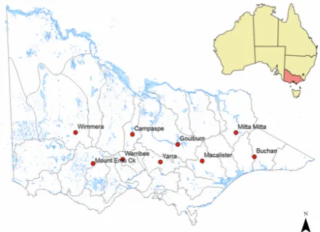
Historical instrumental daily rainfall data was obtained from the Australian Bureau of Meteorology for nine rainfall sta-tions distributed across Victoria, Australia (see Fig. 1). The rainfall gauges were selected to represent nine target catch-ments that are important for water resources management in Victoria. Monthly rainfall totals from January 1948 to April 2006 were used in this study, with months containing more than 5 days of missing data excluded from the analysis. 2.3 Climate indices
2.3.1 ENSO
Fig. 1. Location of rainfall stations used in this study.
Climate Prediction Centre (CPC) is used to provide a rep-resentation of ENSO conditions. The ONI index is de-rived from sea surface temperature (SST) anomalies in the equatorial Pacific Ocean using a 3 month running mean of ERSST.v3 SST anomalies in the Ni˜no 3.4 region (5◦N–5◦S, 120◦–170◦W). Warm (positive) SST anomalies are associ-ated with El Ni˜no events, while La Ni˜na events are typically associated with cold (negative) SST anomalies.
2.3.2 IOD
An index based on SST anomalies over Indonesia (0–10◦S, 120–130◦E) is used in this study to represent climate vari-ability in the Indian Ocean associated with the Indian Ocean Dipole (IOD). This index, known as the Indonesian Index (II), relates to one of the “poles” of the Indian Ocean Dipole as identified by Nicholls (1989) and has been shown to be a good indication of winter rainfall in eastern Australia (Ver-don and Franks, 2005). In fact, this index was found to relate better to east Australian rainfall than other IOD indices such as the Dipole Mode Index (DMI) of Saji et al. (1999). When SSTs are anomalously cool over Indonesia, winter rainfall tends to be lower, while warm SSTs in the same region are related to higher winter rainfalls in eastern Australia. 2.3.3 SAM
The SAM is represented by the monthly mean Antarctic Oscillation (AAO) index, available from NOAA CPC from 1979 to present and from Thompson and Wallace (2000) from 1948–2002. In this study the NOAA CPC version of the AAO is used where it exists (i.e. from 1979) and the Thompson and Wallace (2000) AAO data is used prior to that. Overlapping periods of the two versions of the AAO were compared and the difference was found to be negligi-ble (R2=0.95). The AAO index is constructed by project-ing the daily 700mb height anomalies poleward of 20◦S onto
the loading pattern of the AAO. The loading pattern of the AAO is defined as the leading mode of Empirical Orthogo-nal Function (EOF) aOrthogo-nalysis of monthly mean 700 hPa height during 1979–2000 period.
2.3.4 IPO
Folland et al. (1999) derived an index of IPO variability us-ing a low pass filter of near-global SSTs, while Power et al. (1999) applied a spectral filter with a 13 year cut-off to the raw IPO to generate a smoothed (or slowly varying) IPO timeseries. The smoothed timeries of Power et al. (1999) is used in this study in order to identify epochs of positive and negative IPO.
3 Synoptic typing methodology
The SOM methodology (Kohonen, 1995) is adopted to iden-tify the key regional synoptic patterns driving rainfall vari-ability in Victoria. SOM is a non-linear neural network clas-sification technique developed to recognise relevant struc-tures in complex, high-dimensional data via an unsupervised learning and self adaptation process (Cavazos et al., 2002). SOMs have been described as less complex, more robust and less subjective than more traditional techniques, including cluster analysis and principal component analysis, which are commonly used to identify synoptic patterns (Hewitson and Crane, 2002).
SOMs are essentially a mapping of many vectors onto a two dimensional array of representative nodes (in this case synoptic types) via an unsupervised learning algorithm. The first stage of the SOM is to initialise a specified number of reference vectors. The user defines the number of reference vectors to train the SOM (i.e. the size of the SOM array), which in this application corresponds to the number of syn-optic types. An iterative approach is then used to train the SOM, according to the following process:
1. A sample vector from the input data set is chosen at ran-dom and the best matching node (reference vector) is determined by calculating the minimum Euclidean dis-tance for each of the reference vectors;
2. Once the best matching node is identified for the input vector, the node and those close to it are updated to-wards the input vector;
3. Training continues using multiple iterations, until sTa-ble values are reached (i.e. no further adjustment is made to the reference vector);
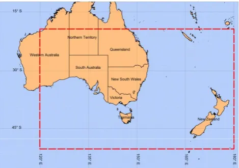
Fig. 2. Region over which the regional synoptic patterns are
anal-ysed in this study.
5. The input data is then classified by locating the best match to the final reference vector. In this case, monthly SLP patterns are matched to the archetypal patterns identified using the SOM to generate a timeseries of synoptic types.
In order to study the regional scale synoptic systems that are important for Victoria, a subset of the global SLP data was extracted to carry out the SOM. This region was cho-sen so as to capture the synoptic patterns that are known to deliver rainfall to Victoria, such as cut-off lows and frontal systems (following Pook et.al, 2006). The location of the SLP field used in this analysis (120◦E–180◦E, 20◦S–50◦S) is shown in Fig. 2.
The size of the SOM array directly influences the range of synoptic patterns represented. A number of array sizes were trialled in order to determine the optimum number of synop-tic patterns. It was determined that a 3 by 4 SOM (i.e. 12 types) was not large enough to adequately identify the sub-tle differences between types that are likely to be important in generating rainfall, however these subtleties were found to be captured by a 4 by 5 SOM (i.e. 20 types). Larger array sizes (e.g. a 5 by 6 SOM) resulted in further refinement of the transitionary synoptic types (resulting in very discrete differ-ences between types) yet did not alter the extreme types. In addition, there was no improvement in the mean error per sample (calculated as the average Euclidian distance between the input vector and the synoptic types it best matches to) by increasing the size of the SOM array beyond 20 types. Given these findings a 4 by 5 SOM was chosen for the synoptic typing performed in this study – this array size satisfactorily captures a range of synoptic patterns with sufficient differ-ences observed between types.
It is possible that the relationship between the regional synoptic patterns and the large-scale climate modes pre-sented in this paper may be sensitive to the size of the SOM
array and/or the resolution of the SLP data and/or the spa-tial region over which the SOM is applied. Therefore, it is acknowledged that further sensitivity analysis is required to determine if/how the relationships identified here change when SOM is applied to different SLP data sets and/or larger/smaller spatial regions than that identified in Fig. 2.
4 Regional-scale climate variability in Victoria 4.1 Identification of 20 key regional synoptic patterns The synoptic typing was carried out using the freely available SOM software (“SOM Toolbox for Matlab 5”, produced by the SOM Toolbox Team, Helsinki University of technology). Twenty synoptic types (using a 4 by 5 grid) were generated using the monthly SLP data, as shown in Fig. 3. By virtue of the method similar types are clustered together in the SOM, with the most dissimilar types located at the far corners of the SOM map.
Figure 3 demonstrates that the 20 synoptic types capture a range of significant synoptic features known to influence the weather of the region. These include the clear seasonal trend in the location and intensity of the semi-permanent Pa-cific and Indian Ocean high pressure systems that are asso-ciated with the Sub-Tropical Ridge (STR). Variability in the strength and location of the east coast trough, located be-tween the two semi permanent high pressure systems, is also evident (i.e. lower left corner of SOM map).
It would be expected that type 1A and to a lesser extent type 1B and 2B would result in high rainfall for the south coast of Victoria. This is due to the northward movement of the high pressure systems and the presence of a pre-frontal trough, which would allow rain producing southern ocean cold fronts to penetrate into southern Victoria (Tapper and Hurry, 1996). While synoptic type 2A appears to be similar to 1A in terms of the location of the high pressure systems, this pattern is unlikely to produce significant rainfall as the pre-fontal trough is located south of Victoria and is much weaker than the trough displayed in type 1A. The blocking high, located in the Southern Ocean for type 2A, is also likely to prevent cold fronts from passing through Victoria.
Fig. 3. 20 key regional synoptic patterns characterised using SOM.
situation is more likely to result in clear (i.e. dry) weather for that region.
Synoptic type 4C exhibits a low pressure trough located offshore, running parallel to the coast, also known as an ‘easterly dip’ (Sturman and Tapper, 2004). The offshore trough is often associated with the development of particu-larly heavy rainfall along the east coast of Australia. Some offshore easterly dips can lead to the development of east coast cyclones (i.e. cut off lows/Tasman lows) during cooler months which are associated with intense rainfall events in Victoria and NSW. Synoptic types 3D and 4D display di-vergence in the isobars located in the Pacific Ocean, east of NSW, which may lead to the development of east coast lows. However, these are unlikely to result in significant rainfall for Victoria as their development is too far to the north.
4.2 Seasonality of the 20 key synoptic types
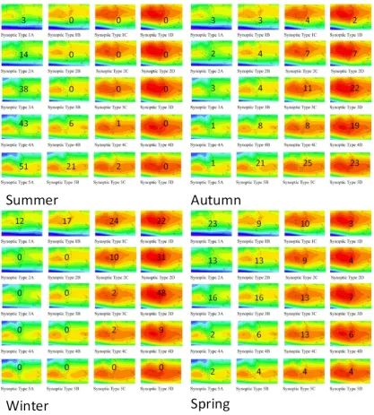
A time-series of synoptic patterns was generated by classify-ing the monthly SLP values (from January 1948 through to April 2007) according to the 20 synoptic types. The classi-fication was achieved by calculating the best matching unit for each month. Figure 4 shows the distribution of synoptic types within each season for the study period (January 1948 to April 2007).
Clear seasonality in the synoptic types is evident in Fig. 4, particularly during the summer and winter months. Winter types tend to be mapped to the top right of the SOM, while summer types tend to map to the bottom left of the SOM. Common winter types (e.g. 1B, 1C, 1D, 2C, 2D, 3D, 4D) are associated with northward movement of the STR and the linking of the Pacific and Indian Ocean high pressure sys-tems. The most common summer types (e.g. 2A, 3A, 4A, 4B, 5A, 5B, 5C) are associated with southward movement of the semi permanent high pressure systems (Pacific and In-dian Ocean high associated with the STR) and a deepening of the east coast low pressure trough.
4.3 Rainfall associated with each of the 20 synoptic types
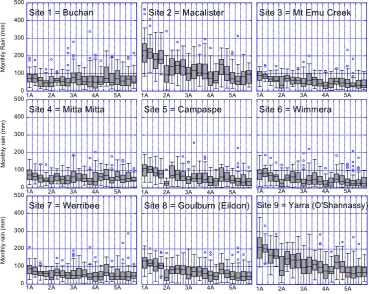
Rainfall distributions associated with each of the 20 synop-tic types were calculated using the monthly rainfall data de-scribed in Sect. 2.2. The rainfall distributions are illustrated in Figure 5.
Fig. 4. Number of times each synoptic type has occurred since 1948 on a seasonal basis. Note: Fig. 3 features a magnified version of the
SOM matrix under laying the frequency of occurrence numbers shown here.
while “dry” types tend to be associated with synoptic pat-terns that map to the bottom two rows of the SOM (i.e. 4A to 5D), with a few noTable exceptions (including the “wet” 4C and 5A types). Generally, the highest rainfall is associated with type 1A, representing a strong pre-frontal trough, with rainfall generated out of the southern Ocean. This result is consistent at all stations except the two far eastern stations, Buchan and Mitta Mitta, where synoptic types 3A (weak east coast trough) and 4C (easterly dip) tend to deliver equally high rainfalls. While type 3A tends to result in high rainfall in eastern Victoria, this system is generally associated with
0 100 200 300 400 500
1A 2A 3A 4A 5A
M o n th ly R a in ( m m )
Site 1 = Buchan
1A 2A 3A 4A 5A Site 2 = Macalister
1A 2A 3A 4A 5A Site 3 = Mt Emu Creek
300 400 500 M o n th ly r a in ( m m )
Site 4 = Mitta Mitta Site 5 = Campaspe Site 6 = Wimmera
1A 2A 3A 4A 5A
Site 9 = Yarra (O'Shannassy)
0 100 200
1A 2A 3A 4A 5A
M o n th ly r a in ( m m )
1A 2A 3A 4A 5A 1A 2A 3A 4A 5A
0 100 200 300 400 500
1A 2A 3A 4A 5A
M o n th ly r a in ( m m )
Site 7 = Werribee
[image:7.595.113.483.65.359.2]1A 2A 3A 4A 5A Site 8 = Goulburn (Eildon)
Fig. 5. Box plots of monthly rainfall associated with each of the 20 synoptic types. Horizontal line within the box indicates the median. Dots
indicate observations that are considered statistical outliers (i.e. extreme events that are greater than 1.5 times the width of the box, which is the difference between the 75th percentile and the 25th percentile of the distribution).
4.4 Relationship with large-scale climate drivers – inter-annual variability
As discussed previously, a number of large-scale climate modes (i.e. ENSO, IOD and SAM) are known to influence the climate of Victoria on an annual to inter-annual timescale. Table 1 shows the average index value of the large-scale cli-mate modes associated with each synoptic type (refer to Sec-tion 2.3 for further informaSec-tion on the ENSO, IOD and SAM indices used in this study).
From the analysis shown in Table 1 it is clear that the cer-tain synoptic types (and therefore weather conditions) are more likely in particular phases of the large-scale climate modes. For example, when the tropical Pacific Ocean is in a La Ni˜na like state (i.e. negative ONI) synoptic patterns 1A, 4A and 5A are most likely – 1A and 5A (and to a lesser degree 4A) are associated with high rainfall in Victoria, par-ticularly for the eastern stations. Conversely, strongly posi-tive ONI conditions (i.e. El Ni˜no) tend to be associated with types 3B, 3D and 4B which in turn are associated with av-erage/below average rainfall across Victoria. There is also a clear relationship between the SAM and the regional synop-tic patterns, with negative SAM linked to synopsynop-tic types lo-cated at the top left of the SOM (i.e. wet types) and positive
SAM linked to those types located at the bottom right (i.e. dry types). It is also interesting to note that synoptic type 1A, associated with the highest rainfall across Victoria, tends to occur when the Pacific Ocean is in a La Ni˜na state, the SAM is negative and warm SSTs dominate the East Indian Ocean. That is, the greatest rainfall is likely to be experienced in Vic-toria when all three climate modes simultaneously occur in their “wet phase”.
Table 1. Average monthly index value (ENSO, IOD, and SAM)
associated with the 20 key regional synoptic types for Victoria.
Synoptic Average Average Average Type ENSO (ONI) IOD (II) SAM (AAO)
1A −0.13 0.24 −0.91
1B 0.10 0.10 −0.64
1C 0.15 0.08 −0.62
1D 0.22 −0.04 0.19
2A 0.16 0.26 −0.82
2B 0.19 0.03 −0.21
2C 0.20 0.01 −0.38
2D 0.25 −0.10 0.70
3A 0.01 0.25 −0.33
3B 0.43 0.16 −0.18
3C 0.02 0.20 0.26
3D 0.30 −0.13 0.45
4A −0.17 0.20 0.94
4B 0.28 0.36 0.44
4C 0.22 0.22 0.17
4D 0.19 0.07 0.50
5A −0.25 0.28 0.11
5B −0.08 0.27 0.39
5C 0.09 0.33 0.36
5D 0.00 0.21 0.34
and Verdon-Kidd, 2009). For example, both types 1A and 2A are associated with strongly negative SAM, however rainfall for type 1A tends to be much greater. This demonstrates that interactions between large-scale climate drivers and regional synoptic patterns must be understood and accounted for in order to better understand (and predict) variability in Victo-ria’s climate.
To further investigate the relationship between the regional synoptic patterns and the large-scale climate modes the oc-currence of each of the 20 regional synoptic patterns were stratified based on the state of the individual modes. Each month from January 1948 to April 2006 was classified as El Ni˜no, La Ni˜na or Neutral based on ONI and the NOAA ENSO classification definition. The same classification pro-cedure was used to classify months as IOD positive, nega-tive or neutral (using the II) and SAM posinega-tive, neganega-tive, or neutral (using the AAO). The number of times each synoptic pattern occurred in combination with an El Ni˜no, La Ni˜na or Neutral event is shown in Fig. 6. Similarly Fig. 7 displays the results for IOD and Figure 8 shows the relationship for SAM.
There is a clear trend towards a higher frequency of synop-tic types 4A and 5A occurring in combination with a La Ni˜na event (as opposed to El Ni˜no) during the summer months. As discussed previously these synoptic patterns are associated with high rainfall for the two eastern stations (i.e. Buchan and Mitta Mitta). Figure 6 also shows that synoptic type 1A
(a very wet type) only occurs in autumn in combination with a La Ni˜na event, indicating that the autumn break (which plays an important role in resulting winter runoff) may be more reliable in a La Ni˜na year. Furthermore, there is an apparent trend towards more of type 3D in winter of an El Ni˜no, which tends to be associated with fairly dry conditions across Victoria.
The IOD is thought to impact rainfall in Australia pri-marily in winter and spring, when the dipole itself is most active (Verdon and Franks, 2005). This also appears to be the case for the regional synoptic patterns, as shown in Fig-ure 7. For example, during these seasons, there is a clear trend towards more frequent wet types (e.g. 1A, 1B and 1C), and an associated decrease in dry type 3D, when the waters around Indonesia are anomalously warm (resulting in a neg-ative dipole).
Across all seasons there is a trend in the relationship be-tween the SAM and the regional synoptic patterns (shown in Fig. 8). That is, the negative phase of the SAM appears to favour the occurrence of synoptic types located at the top left of the SOM (which are generally wet types), while the posi-tive phase tends to be connected to the occurrence of synop-tic patterns located on the bottom right of the SOM (which generally correspond to dry types). This difference is most apparent in the spring and autumn seasons.
4.5 Relationship with large-scale climate drivers – multi-decadal variability
As discussed in the Introduction, the climate of eastern Aus-tralia has experienced a number of multi-decadal shifts (i.e. mid 1940’s and mid 1970’s) in climate which have since been associated with the IPO/PDO. In order to investigate if these multi-decadal shifts have resulted in changes in the regional synoptic patterns, the frequency of types post 1978 (i.e. posi-tive IPO) were compared to the frequency of types during the period 1948–1978 (i.e. IPO negative). The results are shown in Fig. 9.
Fig. 6. Number of times each synoptic type has occurred since 1948 on a seasonal basis, stratified into El Ni˜no (EN), La Ni˜na (LN) and
Neutral (N) phases. Note: Fig. 3 features a magnified version of the SOM matrix under laying the frequency of occurrence numbers shown here.
5 Conclusions
It is clear that Pacific, Indian and Southern Ocean climate variability plays an important role in modulating the regional synoptic systems that deliver rainfall to Victoria. It is also shown that the dominance of the large-scale climate modes (e.g. ENSO, IOD and SAM) varies with season and the re-sulting impact differs in strength from location to location.
The analysis presented here has marked implications in a variety of climate impact related areas, in particular seasonal
Fig. 7. Number of times each synoptic type has occurred since 1948 on a seasonal basis, stratified into IOD positive (+ve), IOD negative
(−ve) and IOD neutral (N) phases. Note: Fig. 3 features a magnified version of the SOM matrix under laying the frequency of occurrence numbers shown here.
weather and the fact that this is not adequately represented in current forecasting schemes (either dynamical models or statistically based) – most likely because the characteristics and interactions associated with the large-scale and regional climate drivers are not yet fully understood.
The results presented in this study demonstrate that any seasonal forecasting framework (dynamical model or statis-tically based) should take into account interactions between all climate phenomena known to affect the predictand. Fore-casting schemes based on large-scale climate indices (e.g.
re-Fig. 8. Number of times each synoptic type has occurred since 1948 on a seasonal basis, stratified into SAM positive (+ve), SAM negative
(−ve) and SAM neutral (N) phases. Note: Fig. 3 features a magnified version of the SOM matrix under laying the frequency of occurrence numbers shown here.
gional climate drivers (using SOM). Future work will utilise insights into the links between large-scale climate modes and regional synoptic patterns to better explain (and predict) local-scale climate variability. Future investigation will also involve analysis of the sensitivity of these results to the use of different SLP data sets and/or alternate synoptic typing techniques (similar to Hope et al., 2006) and/or alternate in-dices to represent large-scale climate modes. It is also worth noting that the methodology used here to identify regionally-specific climate drivers (and their relationships with
[image:11.595.89.510.62.533.2]Fig. 9. Number of times each synoptic type has occurred since 1948 on a seasonal basis, stratified into IPO positive (+ve) and IPO negative
(-ve) phases for (a) summer, (b) autumn, (c) winter, (d) spring.
Edited by: M. Sivapalan
References
Ashok, K., Guan, Z., and Yamagata, T.: Influence of the Indian Ocean Dipole on the Australian winter rainfall, Geophys. Res. Lett., 30, doi:10.1029/2003GL017926, 2003.
Cavazos, T.: Using self-organizing maps to investigate extreme cli-mate events: An application to wintertime precipitation in the Balkans, J. Clim., 13, 1718–1732, 2000.
Cavazos, T., Comrie, A. C., and Liverman, D. M.: Intraseasonal variability associated with wet monsoons in southeast Arizona, J. Clim., 15, 2477–2490, 2002.
Chiew, F. H. S., Piechota, T. C., Dracup, J. A., and McMahon, T. A.: El Nino Southern Oscillation and Australian rainfall, streamflow and drought - links and potential for forecasting, J. Hydrol., 204, 138–149, 1998.
Drosdowsky, W.: The latitude of the subtropical ridge over East-ern Australia: The L index revisited, Int. J. Climatol., 25, 1291– 1299, 2005.
Erskine, W. D. and Warner, R. F.: Geomorphic effects of alternating flood and drought dominated regimes on a coastal NSW river, in: Fluvial Geomorphology of Australia, Academic Press, Sydney, Australia, 223–244, 1988.
Folland, C. K., Parker, D. E., Colman, A. W., and Washington, R.: Large scale modes of ocean surface temperature since the late nineteenth century, in: Beyond El Nino: Decadal and Inter-decadal Climate Variability, Springer, Berlin, Germany, 73–102, 1999.
Franks, S. W. and Kuczera, G.: Flood frequency analysis: Evidence and implications of secular climate variability, New South Wales, Water Resour. Res., 38(5), doi:10.1029/2001WR000232, 2002.
Hewitson, B. C. and Crane, R. G.: Self-organizing maps: applica-tion to synoptic climatology, Clim. Res., 22, 13–26, 2002. Hope, P. K., Drosdowsky, W., and Nicholls, N.: Shifts in the
synop-tic systems influencing southwest Western Australia, Clim. Dy-nam., 26, 751–764, 2006.
Kiem, A. S. and Verdon-Kidd, D. C.: Climatic drivers of Victorian streamflow – is ENSO the dominant influence?, Austr. J. Water Resour., 13(1), 2009.
Kohonen, T.: Self-organizing maps, Springer, New York, USA, 501 pp., 1995.
Mantua, N. J., Hare, S. R., Zhang, Y., Wallace, J. M., and Francis, R. C.: A Pacific decadal climate oscillation with impacts on salmon production, B. Am. Meteor. Soc., 78, 1069–1079, 1997. McMahon, T. A., Finlayson, B. L., Haines, A. T., and Srikanthan,
R.: Runoff variability: a global perspective, in: Influence of Cli-mate Change and Climatic Variability on the Hydrologic Regime and Water Resources, vol. 168. International Association of Hy-drological Sciences, Wallingford, England, UK, 3–11, 1987. Meneghini, B., Simmonds, I., and Smith, I. N.: Association
be-tween Australian rainfall and the Southern Annular Mode, Int. J. Climatol., 27, 109–121, 2007.
Murphy, B. F. and Timbal, B.: A review of recent climate variability and climate change in southeastern Australia, Int. J. Climatol., 28, 859–879, 2007.
Nicholls, N.: Sea surface temperatures and Australian winter rain-fall, J. Clim., 2, 965–973, 1989.
Nicholls, N., Drosdowsky, W., and Lavery, B.: Australian rainfall variability and change, Weather, 52, 66–72, 1997.
Pook, M. J., McIntosh, P. C., and Meyers, G. A.: The synoptic decomposition of cool-season rainfall in the southeastern Aus-tralian cropping region, J. Appl. Meteor. Clim., 45, 1156–1170, 2006.
Power, S., Tseitkin, F., Torok, S., Lavery, B., Dahni, R., and McA-vaney, B.: Australian temperature, Australian rainfall and the Southern Oscillation, 1910-1992: coherent variability and re-cent changes, Australian Meteorological Magazine, 47, 85–101, 1998.
Reusch, D. B., Alley, R. B., and Hewitson, B. C.: North Atlantic cli-mate variability from a self-organizing map perspective, J.. Geo-phys. Res., 112, D02104, doi:02110.01029/02006JD007460, 2007.
Ropelewski, C. F. and Halpert, M. S.: Global and Regional Scale Precipitation Patterns Associated with the El Ni˜no/Southern Os-cillation, Mon. Weather Rev., 115, 1606–1626, 1987.
Saji, H. H., Goswami, B. N., Vinayachandran, P. N., and Yamagata, T.: A dipole mode in the tropical Indian Ocean, Nature, 401, 360–363, 1999.
Stone, R. and Auliciems, A.: SOI Phase relationships with rainfall in eastern Austalia, Int. J. Climatol., 12, 625–636, 1992. Sturman, A. and Tapper, N.: The Weather and Climate of Australia
and New Zealand, Oxford University Press, Melbourne, Victoria, Australia, 2004.
Tapper, N. and Hurry, L.: Australia’s Weather Patterns – An In-troductory Guide, Dellasta Pty Ltd., Mount Waverly, Victoria, 1996.
Thompson, D. W. J. and Wallace, J. M.: Annular modes in the extra-tropical circulation, part I: month-to-month variability, J. Clim., 13, 1000–1016, 2000.
Timbal, B. and Jones, D. A.: Future projections of winter rainfall in southeast Australia using a statistical downscaling technique, Clim. Change, 86, 165–187, 2008.
Verdon, D. C. and Franks, S. W.: Indian Ocean sea surface tempera-ture variability and winter rainfall: Eastern Australia, Water Res. Res., 41, W09413, doi:09410.01029/02004WR003845, 2005. Verdon, D. C. and Franks, S. W.: Long-term behaviour of ENSO:
Interactions with the PDO over the past 400 years inferred from paleoclimate records, Geophys. Res. Lett., 33, L06712, doi:10.1029/2005GL025052, 2006.
Verdon, D. C., Wyatt, A. M., Kiem, A. S., and Franks, S. W.: Multi-decadal variability of rainfall and stream-flow – Eastern Australia, Water Res. Res., 40, W10201, doi:10210.11029/12004WR003234, 2004.
Wright, W. J.: A synoptic climatological classification of winter precipitation in Victoria, Australian Meteorological Magazine, 37, 217–229, 1989.