https://doi.org/10.5194/hess-21-5401-2017 © Author(s) 2017. This work is distributed under the Creative Commons Attribution 3.0 License.
Field-scale water balance closure in seasonally frozen conditions
Xicai Pan1,2, Warren Helgason3,1, Andrew Ireson4,1, and Howard Wheater1
1Global Institute for Water Security, University of Saskatchewan, Saskatoon, SK, Canada 2State Key Laboratory of Soil and Sustainable Agriculture, Institute of Soil Science, Chinese Academy of Sciences, Nanjing, China
3Civil and Geological Engineering, University of Saskatchewan, Saskatoon, SK, Canada 4School of Environment and Sustainability, University of Saskatchewan, Saskatoon, SK, Canada Correspondence to:Warren Helgason (warren.helgason@usask.ca)
Received: 26 May 2016 – Discussion started: 16 June 2016
Revised: 25 July 2017 – Accepted: 25 July 2017 – Published: 1 November 2017
Abstract. Hydrological water balance closure is a simple concept, yet in practice it is uncommon to measure every significant term independently in the field. Here we demon-strate the degree to which the field-scale water balance can be closed using only routine field observations in a season-ally frozen prairie pasture field site in Saskatchewan, Canada. Arrays of snow and soil moisture measurements were com-bined with a precipitation gauge and flux tower evapotran-spiration estimates. We consider three hydrologically distinct periods: the snow accumulation period over the winter, the snowmelt period in spring, and the summer growing season. In each period, we attempt to quantify the residual between net precipitation (precipitation minus evaporation) and the change in field-scale storage (snow and soil moisture), while accounting for measurement uncertainties. When the resid-ual is negligible, a simple 1-D water balance with no net drainage is adequate. When the residual is non-negligible, we must find additional processes to explain the result. We identify the hydrological fluxes which confound the 1-D wa-ter balance assumptions during different periods of the year, notably blowing snow and frozen soil moisture redistribution during the snow accumulation period, and snowmelt runoff and soil drainage during the melt period. Challenges associ-ated with quantifying these processes, as well as uncertain-ties in the measurable quantiuncertain-ties, caution against the com-mon use of water balance residuals to estimate fluxes and constrain models in such a complex environment.
1 Introduction
Water balance closure has been described as the holy grail of scientific hydrology (Beven, 2006). Beven suggests that the most important problem in hydrology in the 21st cen-tury is providing the techniques to measure integrated fluxes and storages on useful scales. In the current paper, we de-fine the problem of water balance closure as that of inde-pendently quantifying each term in the water balance equa-tion, such that the changes in storage within a specified do-main and over some time interval are adequately balanced by the net fluxes into or out of that domain over the same time interval. As simple as this concept is, it has proven to be extremely hard to achieve in field studies. For example, Mazur et al. (2011) reported a water balance closure study for a well-characterized, intensively monitored artificial catch-ment and were unable to close the water balance due to their inability to quantify evapotranspiration and changes in stor-age. Natural heterogeneity of both water fluxes and moisture states, which can vary on spatial and temporal scales that are beyond (or beneath) our measurement capabilities, can make the task of observing complete water balance closure seem like an enigmatic pursuit.
northern portion of the Great Plains region of North Amer-ica. The hydrology of this region is markedly influenced by the regional climate and geology and at first glance appears to have a relatively simple water balance. Much of the rain-fall occurs during the growing season and is consumed by evapotranspiration, resulting in very little surface runoff. Ex-tensive past glaciations have blanketed the region with a thick compacted till which has very low permeability (Keller et al., 1989), resulting in relatively small interactions between the surface water and the underlying groundwater regime (van der Kamp and Hayashi, 2009). As such, the water balance in this region is conceptualized to be dominated by vertical ex-changes of precipitation and evapotranspiration between the soil and the atmosphere.
However, certain characteristics of the prairie region also make the hydrology complex and are likely to confound sim-ple 1-D assumptions regarding the water budget. The region is seasonally frozen, with long winters (4–6 months), fea-turing many cryosphere-dominated hydrological processes. Approximately one-third of annual precipitation is snowfall, which is subject to extensive wind redistribution throughout the landscape (Pomeroy et al., 1993; Pomeroy and Li, 2000), resulting in a spatially variable water input. During the spring melt, spatially variable surface albedos and heat advection from snow-free to snow-covered areas can cause differential rates of snowmelt (Shook et al., 1993; Liston, 1995). More-over, infiltration into frozen soil has complex dependencies upon the antecedent moisture, the rate of melt, and local to-pography (Gray et al., 2001), resulting in a highly variable spatial infiltration pattern (Hayashi et al., 2003; Lundberg et al., 2016). Due to these factors, the annual snowmelt event typically produces 80 % or more of the annual local surface runoff (Gray and Landine, 1988). The hydrological complex-ity of the landscape is also largely influenced by glacial and post-glacial geomorphological processes, which have im-parted a tremendous degree of heterogeneity. Morainal de-posits, comprised of a variable mix of soil textures, are often topographically indeterminate and consist of areas which are internally drained and infrequently contribute to stream flow (Zebarth and de Jong, 1989; Shaw et al., 2012).
While observations of all of the hydrological fluxes and states on large, i.e. useful (Beven, 2006), scales are desir-able, current measurement approaches do not yet fully per-mit this. The evaporative flux can be measured over reason-ably large scales (on the order of hundreds of metres) us-ing the eddy covariance technique, whereas the soil moisture status and bottom drainage fluxes can generally only be mea-sured on point scales. Recent advances in remotely sensed soil moisture, such as the ground-based cosmic ray neutron probe (Zreda et al., 2008) or satellite-based sensors such as those used by the Soil Moisture and Ocean Salinity (SMOS) mission (Kerr et al., 2010) or the Soil Moisture Active Pas-sive (SMAP) mission (Entekhabi et al., 2010), can retrieve soil moisture estimates over hundreds of metres to tens of kilometres. However, these observations are limited to the
near surface, and need to be depth-scaled to the root zone to be suitable for water balance studies (Peterson et al., 2016). Adequately capturing field-scale variability using point-scale measurement techniques requires a large number of samples (e.g. Grayson and Western, 1998; Famiglietti et al., 2008; Brocca et al., 2010).
The objective of this paper is to explore how well the wa-ter balance can be closed using only routine field observa-tions in a seasonally frozen environment. We use a well-instrumented field site to quantify the magnitude of the water balance components as they vary across three distinct sea-sons in the prairies on field scale. We start with a conceptual model of all of the dominant hydrological processes active at the site, from which we construct a water balance equation. We designed a simple field experiment to measure the com-ponents of the water balance that can be measured in a rou-tine, if labour-intensive, manner on field scale. We performed an uncertainty analysis on each measurement, accounting for instrument error and sampling error. We evaluate the validity of treating the problem as 1-D in different seasons, and the value of using water balance residuals to estimate fluxes and constrain models.
2 Methods
2.1 Field-scale water budget
We consider field scale to represent an area on the order of 500 m×500 m, from the ground surface to a depth of 1.6 m. This was the depth range that we were able to install neutron probe access tubes to monitor, and is deep enough to cap-ture all of the significant soil moiscap-ture dynamics at our site. On this scale, storage terms include surface storage (1Ss), which includes snow and ponded water, and subsurface (va-dose zone) storage (1Sv), which is liquid or solid (ice) soil moisture integrated over the root zone (taken to be 1.6 m). The field-scale vertical water balance can hence be expressed for the surface as
1Ss=P−ES−I−G−O, (1)
for the subsurface as
1Sv=I−EB−D, (2)
and for the overall field scale as
1ST=1SS+1Sv=P−E−O−G−D, (3) where all terms are in units of millimetres, andP is precip-itation (solid and liquid phases);I is infiltration;E,ES, and
field domain;Gis net drifting snow over the field domain; andDis vertical soil drainage at 1.6 m depth.
The water table is located 3–5 m belowground surface de-pending on location (the water table is shallower in topo-graphic depressions) and time of year (the water table is shal-lowest in the earlier summer after the melt period). Water ta-ble dynamics are modest, but there will be lateral saturated flow processes occurring. Since the saturated zone is well below the domain of our water balance, here we only con-sider vertical drainage from the base of our soil layer. Lat-eral unsaturated subsurface flow may occur on local scales due to changes in soil properties, but we do not expect these fluxes to be significant on field scale. Hence, lateral subsur-face fluxes are neglected.
In seasonally frozen environments where winters are long and cold, processes in the summer and winter are markedly different. A water year in this region is typically defined as from November to October, such that snow accumulation and melt occur within the same water year. Annual water bal-ances are useful, but do not elucidate the important seasonal processes – in particular the storage dynamics. For a more rigorous analysis, here we examine the water balance over three distinct seasons: the snow accumulation periodstarts from the first killing frost (<−2◦), and ends at the beginning of snowmelt;the melt period, which in a typical year starts from the peak snowpack and ends when the ground is com-pletely snow-free, typically 2–4 weeks sometime in March, April, or May; andthe growing season, which starts from the end of the melt period and ends with the onset of the snow accumulation period, roughly May to October.
In each period the nature of the individual components of the water budget is different. For example, in the snow ac-cumulation period, surface storage occurs as snow; in the growing season, if it exists at all, it is as ponded water in ephemeral ponds which tend to dry out in early summer; and in the melt period, it is a transition between these two. Snow drift, runoff, and evaporation are typically only significant in the snow accumulation season, the melt period, and the growing season, respectively. This will be discussed in detail in Sect. 4.
2.2 Description of study site
[image:3.612.307.550.64.352.2]The instrumented field site (51◦2205400N, 106◦2405700W) lies within a gauged sub-basin (Fig. 1) of the Brightwater Creek watershed, which is a sub-basin of the South Saskatchewan River Basin. The gross area of the sub-basin defined by the Water Survey Canada gauge (05HG002) is 900 km2, while the effective basin area, or that which would be expected to contribute flow to the main stream channel during a flood with a return period of 2 years (Martin, 2001), is just 282 km2 (Fig. 1a). Mean annual precipitation is about 330 mm (2009– 2014), of which about 70 mm typically falls as snow. Mean annual yield via streamflow in the Brightwater Creek wa-tershed is 4.95×10⁶m3(1983–2013), equivalent to 5.5 mm
Figure 1. Brightwater Creek sub-basin in Saskatchewan River Basin (effective drainage area shown by hatching) and locations of measurements.(a)Flux tower (triangle) and the schematic distribu-tion of neutron monitoring locadistribu-tions (right upper corner); red cir-cle: discharge measurement location.(b)Measurements along the long transect shown in the right upper corner of(a)include: neu-tron probe access tubes (N5, N4, N3, N2, N1, M0, S1, S2, S3, S4, S5, S6, S7, S8), snow survey points (the same location as the tubes), and three 6 m piezometer boreholes (no. 1, no. 2 and no. 3).
over the gross drainage area or 17.6 mm over the effective drainage area. Annual runoff is therefore small by either measure. Streamflow is intermittent, and in most years only occurs following snowmelt. The mean temperature in Jan-uary and July is −12.9 and 18.8◦C, respectively. The re-gional landscape consists of gently sloping glacio-lacustrine plains surrounded by moraine deposits that have a rolling knob- and kettle-type topography (Miller et al., 1985). The soils in the region are mainly Solonetzic and Chernozemic, and are mapped as Bradwell and Asquith associations as de-scribed by Ellis et al. (1968).
communi-ties are interspersed in a spatial pattern on the order of tens of metres. The texture of the soils within the study area ranges from loam to clay loam.
2.3 Instrumentation
A variety of measurements were used to characterize the field-scale water balance from 1 November 2012, reported here until 31 October 2014. The total evaporation flux,
E (mm), was obtained using the eddy covariance tech-nique. This consisted of a Campbell Scientific CSAT3 sonic anemometer and a Campbell Scientific KH20 krypton hy-grometer mounted on a scaffold tower located in the center of the study area. The instruments were mounted at a height of 4.85 m aboveground and had a representative measurement fetch of approximately 500 m (Burba, 2013). Raw data were collected at a rate of 10 Hz, and latent heat fluxes (QE=λE, where λ is the latent heat of vaporization or sublimation) and sensible heat flux (QH) fluxes were calculated using Licor EddyPro software (www.licor.com/eddypro). Gaps in the flux data were filled using the Kalman filter and a dy-namic linear regression for recursive parameter estimation developed by Young and coworkers (Young, 1999; Young and Pedregal, 1999; Young et al., 2004), based on the re-lationship between latent heat flux, available energy, and vapour pressure deficit. This gap-filling approach was evalu-ated and recommended by Alavi et al. (2006) for filling gaps in latent heat flux data.
The available energy, consisting of the net radiation flux (QNR)and the ground heat flux (QG)was measured at two locations within the eddy-covariance measurement footprint: representing grass and brush surfaces. At the scaffold tower (grass surface), net radiation fluxes were measured using a Kipp and Zonen CNR1 four-component radiometer, whereas net radiation fluxes at an auxiliary tripod (brush cover) lo-cated approximately 100 m from the scaffold were measured with a Hukseflux NR01 four-component radiometer. At both locations two heat flux plates (Radiation Energy Balance Systems model HFT3) were installed at a depth of 8 cm and were laterally separated by∼1 m. In order to calculate energy storage in the soil layer above the heat flux plates (1SG), a single volumetric water content sensor (Campbell Scientific CS650 dielectric permittivity sensor) was installed at 5 cm depth, and a pair of averaging thermocouples were in-stalled at 4 cm depth. The available energy, calculated as the net radiation flux minus (plus) the amount of energy trans-ferred into (from) the soil, was averaged between the two locations.
The energy balance closure ratio (EBR), EBR= 6 (QE+QH)
6 (QRN−QG−1SG)
, (4)
was evaluated for each day of the growing season, which gave an average closure fraction of 0.72 and 0.74 in 2013 and 2014, respectively. These biases were corrected by
forc-ing energy balance closure usforc-ing the measured Bowen ratio (cf. Twine et al., 2000; Barr et al., 2012) on a daily basis, which increased the measured seasonal evaporation fluxes by 39 and 35 % in 2013 and 2014, respectively. Biases for the other seasons were not corrected since the evaporation fluxes over the frozen ground surface were very small, and the turbulent heat fluxes are much more uncertain over snow (Helgason and Pomeroy, 2012).
Precipitation (mm) was measured by a Geonor T200-B weighing gauge. Biases in solid precipitation (i.e. snow) measurements were corrected for undercatch using a catch efficiency relationship with wind speed (Smith, 2008), and for liquid precipitation (i.e. rain) we assume a catch effi-ciency of 95 % for all rainfall measurements (Devine and Mekis, 2008). Precipitation bias-correction leads to an in-crease in measured precipitation of 19 and 13 % in 2013 and 2014, respectively.
Root zone soil water content and snowpack depth and den-sity were measured at point locations in a crosshair pattern, comprising two perpendicular transects, centered on the flux tower (shown in the upper right corner of Fig. 1a). Water content was measured by a down-hole neutron moisture me-ter, model CPN 503DR Hydroprobe (CPN International Inc., Concord, CA). The blue pins are the neutron probe reading locations installed in June 2012, and the yellow pins show new locations added in summer 2013. Volumetric soil mois-ture content (liquid water+ice) was measured at depth in-tervals of 0.2 m, from 0.2 to 1.6 m belowground. Due to the problem of surface loss of neutrons, no readings shallower than 0.2 m were taken, meaning we may underestimate the changes in water content at the top of the soil profile. The change in soil water storage,1Sv, was calculated as the dif-ference between any two moisture surveys, which were con-ducted with a time interval of around 2 weeks in the unfrozen period, and 2–3 times during the frozen period. Snowpack distribution along the long transect was investigated with a series of snow surveys during the snow covered period in late winter–spring of 2013 and 2014. Snow depth was mea-sured at a distance interval of about every 2.0–3.0 m, and snow samples were taken from the neutron probe locations, i.e. every 50 m, using a core sampler (ESC30, Environment Canada, Canada) to determine snow density and calculate snow water equivalent (SWE). The change in snow water storage,1Ss, was calculated as the difference in the mean SWE between any two sampling dates. The topography of the long transect from northwest to southeast is shown in Fig. 1b.
flux tower, using the graphical method for estimation of baro-metric efficiency proposed by Gonthier (2007).
Soil temperature was measured using Stevens Hydro-probes at three profiles, co-located with the piezometers. At profile no. 1 (Fig. 1b) five probes were installed, at depths of 0.05, 0.2, 0.5, 1.0, and 1.5 m belowground, and at the other two profiles seven probes were installed, at depths of 0.05, 0.2, 0.5, 0.75, 1.0, 1.3, and 1.6 m belowground. Measure-ments were recorded every 30 min. The depth of the freezing front as a function of time was calculated by interpolating the 0◦C line from the soil temperature measurements.
2.4 Uncertainty assessment
We performed a quantitative uncertainty analysis of all of the measured terms in our water balance assessment. We ex-pect uncertainties in our measurements of precipitation and evapotranspiration to be dominated by measurement errors. Conversely, we expect uncertainties in our measurements of soil moisture and snowpack to be dominated by sampling errors. These four terms make up a naïve, 1-D, water bal-ance, where the net precipitation (defined asP−E)equals the total change in storage (1Ss+1Sv). The water balance residual,R, is given by the following:
R=P−E−1Ss−1Sv. (5)
IfRis negligible, we can say the 1-D water balance is ap-propriate. IfRis significantly larger than zero in any period, we must expect one or more other fluxes from Eqs. (1–3) to be significant in that period. We seek to quantify an er-ror bound for each term,±ε, and combining these errors by summing in quadrature to establish an error bound for the residual, εR, given by the following (Coleman and Steele, 1989):
εR= q
(εP)2+(εE)2+ εSs 2
+ εSv 2
. (6)
The error bounds for each measurement term are described in the following paragraphs. In all cases, we concentrate on quantifying the largest, most dominant, source of uncertainty. Precipitation. With respect to the weighing gauge used here (Geonor T-200b), instrument error is actually quite small, i.e. the manufacturer provides an accuracy esti-mate of 0.1 % full scale (which is only 0.6 mm). Similarly, Duchon (2008) presents an example validation of the factory calibration equation, demonstrating that minor calibration er-rors typically introduce small biases (< 1 %) which occur at small or large bucket volumes. However, comparatively large biases can occur due to wind-induced undercatch of solid precipitation (Goodison et al., 1998). In this study, we correct for this bias using the relationship provided by Smith (2008), which predicts the gauge catch efficiency as a function of wind speed. Details on the correction method, and its rel-ative importance in the prairie environment can be found in
Pan et al. (2016). Owing to experimental difficulties in devel-oping a catch efficiency equation, there is considerable (but not quantified) uncertainty which must be introduced when applying the correction factor (this is inferred by the rela-tively large scatter in Figs. 4 and 6 of Smith, 2008). Thus we consider the dominant uncertainty of the winter precipitation measurements to be the wind-induced undercatch (bias)± a random uncertainty associated with the applied correction factor. In order to estimate the latter, we obtained the original data from Smith (2008) and calculated the prediction inter-vals (95 %) on the catch efficiency equation. These were then used to estimate the random error introduced by applying the correction factor to each snow event for the current study. The cumulative random error for each snow accumulation period was calculated by summing all of the individual event errors in quadrature. Undercatch errors are much larger for solid precipitation compared with liquid precipitation; thus all rainfall values are corrected for an undercatch 5 % bias (Pan et al., 2016). On an annual basis, these systematic cor-rections result in an increase in precipitation of 47 mm in 2013 and 44 mm in 2014. It is hard to rigorously quantify any additional random errors in the precipitation measure-ment, so we have assumed random errors of 10 % of daily precipitation.
Evaporation.Measurements of evaporation using the eddy covariance technique may be subject to random measurement error as well as systematic errors due to instrument limi-tations, unmet theoretical assumptions, or processing issues (Richardson et al., 2012). In this study we deal with random errors in an overly simplistic manner by assuming that they are 10 % of the daily E. While this may be the approximate order of magnitude for water vapour flux random errors (e.g. Moncrief et al., 1996; Litt et al., 2015), the approach is only justified in this case by the fact that the random errors are dwarfed by the systematic errors. While some systematic er-rors are corrected for during flux processing (e.g. sensor sep-aration, density fluctuations, high-frequency losses) it is clear that there are other systematic errors that are not accounted for. We deal with these by forcing energy balance closure (Eq. 4), which, on an annual basis, resulted in an additional 80 mm of evapotranspiration in 2013 and 95 mm in 2014.
hetero-Figure 2.Fluctuation of the major variables in vadose zone hydrology during the years of 2013 and 2014.(a)Precipitation and snowpack depth measured at the flux tower.(b)Yearly cumulative change of evapotranspiration (E) and precipitation (P).(c)Average soil water storage change in shallow vadose zone (neutron probe data).(d)Surficial soil freezing above groundwater table at three locations (P1, P2, and P3). (e)Seasonal fluctuation of groundwater level. Black and red dashed lines are the start and end of the snowmelt periods.
geneous snow field. The confidence associated with this es-timate is rarely reported. In this study, we use a bootstrap sampling technique (described below) to assess the standard error (SE) of the mean snow depth and mean snow density, which were propagated to obtain the SE for the mean areal SWE. The 95 % confidence intervals were then calculated as 1.96×SE. An important assumption of this approach is that the snow density samples, collected on 50 m spacing, can be considered random. For shallow prairie snowpacks, random behaviour is found after length scales of around 30 m (Shook and Gray, 1996).
Soil moisture.Soil moisture measurements obtained using the neutron thermalization technique are subject to instru-ment errors, calibration errors, depth integration errors, and spatial sampling errors (Vandervaere et al., 1994). Similar to the estimation of SWE, we consider limited sampling in space to be the largest form of uncertainty in estimating soil moisture changes. Some of the instrument and calibration er-rors are minimized when changes in soil moisture are of in-terest rather than the total soil moisture storage (Vandervaere et al., 1994). In order to calculate the 95 % confidence
inter-vals around the spatial mean soil moisture change, we used a bootstrap resampling technique (e.g. Cosh et al., 2004) in which the soil moisture change was resampled 5000 times (with replacement). The standard error of the areal mean was obtained as the standard deviation of all of the boot-strapped mean estimates. In cases where the data were nor-mally distributed, the 95 % confidence interval was taken as ±1.96×SE. In the event where the data were not normally distributed, the confidence intervals were found using a per-centile method.
3 Results and discussion
[image:6.612.159.439.66.383.2]Table 1.Components of the water balance for each season in 2013 and 2014 (see Eq. 5 and related discussion in the text for symbols).
Observations (mm) Residual (mm)
Seasons P E 1Ss 1Sv R
Snow Accumulation 2013 (1 Nov–8 Apr)
72±2 14±1 97±10 24±11 −63±15
Melt 2013 (9 Apr–6 May )
10±1 16±1 −97±10 54±26 37±28
Grow 2013 (7 May–6 Nov)
220±6 255±2 0 −75±24 40±25
Snow Accumulation 2014 (7 Nov–2 Apr)
72±4 10±1 62±7 13±5 −13±10
Melt 2014 (3–24 Apr )
33±2 15±1 −62±7 30±28 50±29
Grow 2014 (25 Apr–22 Oct )
281±6 343±3 0 −30±17 −32±18
Figure 3.Spatio-temporal variation of snowpack depth along the snow survey transect in 2013(a)to 2014(b).
snowfall was coincidentally the same in both years: 72 mm. Rainfall was 230 (2013) and 314 mm (2014). The sum of evaporation, transpiration, and sublimation was 285 (2013) and 368 mm (2014). Both years had low measured sublima-tion: 14 (2013) and 10 mm (2014). Most evapotranspiration occurred in June, July and August. Water year 2013 was typ-ical for the region in that soil moisture was recharged follow-ing snowmelt, and then experienced dryfollow-ing over the summer months asEexceeded precipitation. Water year 2014 experi-enced a wet May–June, so that soil moisture decreases were delayed to the latter part of the summer. In the following sec-tions, the dominant hydrological processes and water balance closure for each of the three seasons are described.
3.1 Snow accumulation period
Figure 4. Comparison of measured solid precipitation, bias-adjusted precipitation, and measured snow on the ground during the snow accumulation period in hydrological years of 2013 (a)and 2014(b). Note that the error bars indicate the 95 % confidence in-tervals of the measured SWE.
results in a net influx or efflux to a particular site generally depends on the relative height of the local and surrounding vegetation, which can trap snow (Pomeroy et al., 1993). Tak-ing sublimation losses into account, Table 1 shows that in 2013 there was markedly more snow on the ground (72 mm SWE) than there wasP −E(58 mm), while in 2014 the two matched closely (both 62 mm). This suggests that in 2013 there was a net contribution of blowing snow to the pasture, meaning that the vegetation within the pasture (grass and shrubs) was more effective at trapping blowing snow than adjacent cropped fields (shorter stubble, usually less than 15 cm). In 2014 the net effect of blowing snow appears to have been negligible, which is to say that the influx and ef-flux of blowing snow were balanced. The continuous snow water balance through this period is shown in Fig. 4. Here it can be seen that random errors in the accumulated precipita-tion are very small compared with the systematic errors asso-ciated with undercatch of solid precipitation and the variable influence of blowing snow.
[image:8.612.313.541.65.244.2]During the snow accumulation period the soil freezes pro-gressively from the surface downwards. The maximum freez-ing depths were 1.3 (2013) and > 1.6 m (2014), as shown in Fig. 2d. The reasons for the differences in freezing depth are a combination of multiple factors, which are beyond the scope of this study to determine. The important point from a water balance perspective is that in both years there was a non-negligible increase in soil water content over the winter (24±11 mm in 2013 and 10 ±5 mm in 2014, Ta-ble 1). Figure 5 shows the change in root zone water content over the winter (from before soil freeze-up, to just before the soil thawed), from all available neutron probe measure-ments. There were increases in water content over the winter,
Figure 5.Over-winter change in water content with depth below-ground. Symbols indicate the mean over all measurement locations, and bars indicate 95 % confidence intervals. In water year 2013, the pre-freeze measurement was taken on 1 November 2012, and the pre-snowmelt measurement on 22 April 2013. In water year 2014, the pre-freeze measurement was taken on 7 November 2013, and the pre-snowmelt measurement on 3 April 2014. Note that the mea-surements were taken at 20 cm depth intervals, but are plotted here as offset±2 cm for clarity.
with larger increases nearer to the surface. The variability of change in soil water content also increases significantly nearer the surface, which implies that the wetting process is non-uniform across the field. Under frozen conditions the water content of the root zone can potentially increase due to infiltration of mid-winter snowmelt events (uncommon, but not unheard of in this environment), or by upward migra-tion caused by freezing-induced hydraulic gradients (Hoek-stra, 1966; Gray and Granger, 1986). It should be noted that the first set of soil moisture measurements in 2013 did not coincide with the peak SWE survey and the end of the accu-mulation period (8 April), but rather occurred on 22 April, so it is possible that some melting snow had infiltrated by that date. During the defined snow accumulation periods, there were no observations of mid-winter melt events in this period (i.e. the temperature did not significantly rise above zero), so we do not believe significant infiltration occurred, and up-ward moisture redistribution is a more plausible explanation. Note that the water table dropped through the winter (Fig. 2), which could also be partly due to upward water migration (Gray and Granger, 1986; Butler et al., 1996; Iwata et al., 2010).
Figure 6. Contrasting snowmelt processes in 2013 and 2014. (a) Snowpack depth. (b) Hydrograph of the Brightwater Creek. (c)Snowfall and rainfall with 10-day interval during melt period.
been given enough attention in the past. We cannot easily measure the fluxes (namely soil drainage,D, which must be negative, and blowing snow,G) needed to close a water bal-ance which would corroborate these changes in storage. If the surface water balance (Eq. 1) is considered separately, the residualRsbecomes smaller (39±10 mm in 2013, 0±7 mm in 2014). This approach can be justified if there is no infil-tration in the snow accumulation period, in which case we attribute the imbalance to the addition of snow blowing onto the field.
3.2 Melt period
The observed timing and magnitude of snowmelt and dis-charge in Brightwater Creek (measured at gauging station 05HG002) in 2013 and 2014 are compared in Fig. 6. Runoff from our field site may or may not have directly contributed to this watershed-scale discharge (see the effective area in Fig. 1a), but the local infiltration and runoff behaviour can still explain the differences seen on the larger scale. The tim-ing of peak discharge in both years is consistent with the timing of the depletion of the snowpack by melting. How-ever, the magnitude of the peak discharge in 2014 is much bigger than that in 2013. Snowpack depths were comparable (Fig. 6), but field-average SWE was significantly higher in 2013 (Table 1), which indicates there is some complex be-haviour in terms of the runoff generation mechanism, which we explore here. In both years, there was a large negative water balance residual, meaning melt from the snowpack
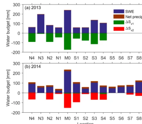
ex-Figure 7.Spatio-temporal variations of soil water storage change in the shallow vadose zone along the Neutron Probe transect dur-ing the melt period (between black and red dashed lines in Fig. 2). SWE: measured maximum snow storage; net precipitation: cumula-tive difference between precipitation and evapotranspiration;1Sv1 and 1Sv2: soil water storage change during post-snowmelt and post-thaw periods.
ceeded the increase in soil moisture, and hence water was lost from the domain, most likely as runoff,O(but possibly also as drainage,D). Peak SWE and melt period changes in root zone soil moisture were measured at coincident points on the transect (Fig. 1b), and the results are shown in Fig. 7 (note that the transect was extended in 2014). In this figure we show the peak SWE and the additional rain that fell dur-ing the melt period as inputs (positive), and the increases in soil moisture (shown as negative numbers) are shown sep-arately for the snowmelt period (1SV1)and the subsequent snow-free soil thaw period (1SV2), which takes considerably longer to complete (Fig. 2). The spatial patterns of snowmelt infiltration are generally consistent between years. More no-table is the difference in timing of the increases in soil mois-ture: in 2013 all of the infiltration occurred while the soils were still frozen, whereas in 2014 there was very little in-filtration into frozen soils, and most of the inin-filtration oc-curred after the soil had thawed. In 2013 there was 54 mm of infiltration of snowmelt, while in 2014 the 30 mm of in-filtration was likely mainly due to rainfall during the late melt period (33 mm). In 2013 we see a runoff residual of 37±28 mm, equivalent to a snowmelt runoff ratio of 38 %, while in 2014 the smaller SWE led to a larger runoff resid-ual of 50±29 mm, equivalent to a snowmelt runoff ratio of 80 %. These residuals are consistent with the observed dif-ferences in basin-scale runoff for 2013 and 2014.
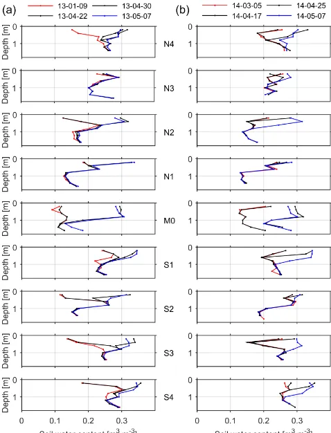
[image:9.612.48.288.65.306.2]Figure 8.Spatio-temporal variation of water content in shallow va-dose zone at different locations (Fig. 1b) along the Neutron Probe reading transect during the pre-melt (red), post-snowmelt (black), and post-thaw (blue) in 2013(a)and 2014(b).
post-snowmelt, and post-thaw conditions are shown in Fig. 8. These observations show the strikingly different antecedent soil moisture conditions in these 2 years, with dry antecedent conditions in 2013 and wet antecedent conditions in 2014. It is well understood (Gray and Landine, 1988; Ireson et al., 2013) that the infiltration capacity of frozen soils de-pends strongly on the antecedent soil moisture. When wetter soils freeze, ice-filled pores develop, giving the soil a rela-tively low infiltration capacity. Drier soils (or more specifi-cally, soils where the largest significant pores, which may be macropores, remain air-filled) can maintain a high infiltra-tion capacity when frozen and the snowmelt infiltrainfiltra-tion can be significant, whilst runoff may be negligible, as in 2013. 3.3 Growing period
Figure 9 shows the observed water budget for the growing period in 2013 and 2014. There is a large, systematic bias in the raw net precipitation, which is caused by the energy balance closure correction for the eddy flux measurement of evaporation. This clearly highlights the importance of mak-ing this correction, whereas the net precipitation was
actu-Figure 9.Comparison of net precipitation (P-E), bias adjusted (en-ergy balance corrected) net precipitation, and cumulative changes in soil moisture during the growing period of hydrological years (a)2013 and(b)2014. Note that the error bars indicate the 95 % confidence intervals of the mean change in soil moisture between adjacent sampling dates.
ally positive prior to adjusting for the lack of energy balance closure. In both years, we seeE exceeding P and the soil moisture being drawn down over the summer, highlighting the importance of snowmelt for sustaining agriculture in this region. In both years, the cumulative bias-adjusted net pre-cipitation is within the confidence intervals of the change in 1SV. It should be noted that the error bars in Fig. 9
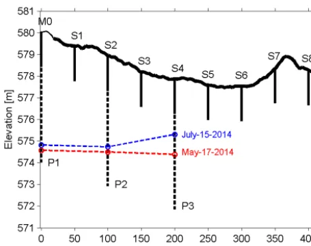
[image:10.612.49.288.66.379.2]Figure 10.Groundwater rise along the slope during the early grow-ing period in 2014.
While we cannot directly measure soil drainage, we have measured the water table response, 3–5 m belowground, which gives some qualitative indication of the timing and relative amount of soil drainage. In 2013, the water table in piezometer 1 (P1) rose steadily during the growing period, though the amount of rise was small,∼20 cm (Fig. 2e). This is consistent with our water-balance-based estimates of soil drainage, which suggested there may have been a small ex-cess in net precipitation through the summer. Combined with the absence of observation of runoff or stream discharge, we can be reasonably confident that this excess did go to soil drainage. In 2014 the water table in P1 rose higher, by ∼50 cm (Fig. 2e), implying that there was significantly more soil drainage this year, which is again consistent with our wa-ter balance in June of 2014. In 2014 two additional piezome-ters (P2 and P3) were available, including one piezometer (P3) located below a topographic depression. The response of these three piezometers is shown in Fig. 10, along with the ground surface elevation. The water table below the de-pression rose markedly more than in the upland piezometers, and peaked much earlier (July). This is consistent with the depression-focused recharge mechanism that has been pro-posed for these environments (Hayashi et al., 2003), though it is important to note that the dominant recharge signal in this study appears to originate from rainfall and not snowmelt.
4 Summary and conclusions
In this study we have used a suite of relatively standard in-strumentation to explore the field-scale water balance. Our findings are of practical importance for those wishing to measure the field-scale water balance, to interpret water bal-ance residuals or use such field-scale observations to cali-brate and/or validate models. Due to the local climate, the
year is split into three periods, each summarized in the fol-lowing paragraphs.
During the winter, i.e. the snow accumulation period, we were unable to close the water balance because we did not directly measure the fluxes of blowing snow or upward soil moisture redistribution, both of which are shown to be sig-nificant. The results of this study emphasize three practical points that should be considered before using similar data to constrain or validate hydrological models: (1) it is critical that solid precipitation records should be adjusted to remove bias due to wind-induced undercatch; (2) a well-timed snow survey to reveal the peak SWE in the snowpack before melt can capture the pre-melt spatial variability, can help negate the requirement to capture blowing snow and sublimation, and can minimize uncertainties in the measured solid phase precipitation; and (3) measuring soil moisture prior to melt, if possible, can be extremely valuable to partition soil mois-ture increases due to over-winter upward redistribution, from increases due to infiltrating snowmelt.
Data availability. All data is available upon request.
Competing interests. The authors declare that they have no conflict of interest.
Acknowledgements. The authors thank Amber Peterson, Bruce Johnson, Dell Bayne, Brenda Toth and Erica Tetlock, who participated in field data collection, as well as Craig Smith and Daqing Yang (National Hydrology Research Centre, Environmental Canada) for providing an unpublished empirical relationship for the Geonor gauge correction. Financial support was provided by the Canada Excellence Research Chair in Water Security, University of Saskatchewan.
Edited by: Ross Woods
Reviewed by: James Buttle, Miles Dyck, and two anonymous referees
References
Alavi, N., Warland, J. S., and Berg, A. A.: Filling gaps in evapotran-spiration measurements for water budget studies: Evaluation of a Kalman filtering approach, Agr. Forest Meteorol., 141, 57–66, 2006.
Barr, A. G., van der Kamp, G., Black, T. A., McCaughey, J. H., and Nesic, Z.: Energy balance closure at the BERMS flux towers in relation to the water balance of the White Gull Creek watershed 1999–2009, Agr. Forest Meteorol., 153, 3–13, 2012.
Beven, K.: Searching for the Holy Grail of scientific hydrology: Qt=(S, R, 1t )Aas closure, Hydrol. Earth Syst. Sci., 10, 609– 618, https://doi.org/10.5194/hess-10-609-2006, 2006.
Brocca, L., Melone, F., Moramarco, T., and Morbidelli, R.: Spatial–temporal variability of soil moisture and its esti-mation across scales, Water Resour. Res., 46, W02516, https://doi.org/10.1029/2009WR008016, 2010.
Burba, G.: Eddy Covariance Method for Scientific, Industrial, Agri-cultural, and Regulatory Applications: A Field Book on Mea-suring Ecosystem Gas Exchange and Areal Emission Rates. LI-COR Biosciences, Lincoln, NE, USA, 331 pp., 2013.
Butler, A. P., Burne, S., and Wheater, H. S.: Observations on freez-ing induced redistribution in soil lysimeters, J. Hydrol. Proc., 10, 471–474, 1996.
Coleman, H. W. and Steele, W. G.: Experimentation and uncertainty analysis for engineers, John Wiley & Sons, New York, 1989. Cosh, M. H., Stedinger, J. R., and Brutsaert, W.: Variability of
sur-face soil moisture at the watershed scale, Water Resour. Res., 40, W12513, https://doi.org/10.1029/2004WR003487, 2004. Devine, K. A. and Mekis, É.: Field accuracy of
Cana-dian rain measurements, Atmos.-Ocean., 46, 213–227, https://doi.org/10.3137/ao.460202, 2008.
Duchon, C. E.: Using vibrating-wire technology for precipitation measurements, in: Precipitation Advances in Measurement, Es-timation and Prediction, edited by: Michaelides, S. C., Springer, Germany, 33–58, 2008.
Ellis, J. G., Acton, D. F., Moss, H. C., Acton, C. J., Ballantyne, A. K., Bristol, O. P., Shields, J. A., Stonehouse, H. B., Janzen, W. K.,
and Radford, F. G.: The Soils of the Rosetown Map Area (72-0 Saskatchewan), Saskatchewan Institute of Pedology Publication S3, Saskatoon, 1968.
Entekhabi, D., Njoku, E. G., O’Neill, P. E., Kellogg, K. H., Crow, W. T., Edelstein, W. N., Entin, J. K., Goodman, S. D., Jackson, T. J., Johnson, J., Kimball, J., Piepmeier, J. R., Koster, R. D., Mar-tin, N., McDonald, K. C., Moghaddam, M., Moran, S., Reichle, R., Shi, J. C., Spencer, M. W., Thurman, S. W., Tsang, L., and Van Zyl, J.: The Soil Moisture Active Passive (SMAP) Mission, P. IEEE, 98, 704–716, 2010.
Famiglietti, J. S., Ryu, D., Berg, A. A., Rodell, M., and Jackson, T. J.: Field observations of soil moisture vari-ability across scales, Water Resour. Res., 44, W01423, https://doi.org/10.1029/2006wr005804, 2008.
Farnes, P., Goodison, B., Peterson, N., and Richards, R.: Proposed metric snow samplers, paper presented at 48th Western Snow Conference, 107–119, 1980.
Farnes, P. E., Goodison, B. E., Peterson, N. R., and Richards, R. P.: Metrication of Manual Snow Sampling Equipment, Final Report, Western Snow Conference, Spokane, Washington, 106 pp., 1983. Gonthier, G. J.: A graphical method for estimation of barometric efficiency from continuous data-concepts and application to a site in the Piedmont, Air Force Plant 6, Marietta, Georgia, US Geol. Surv. Sci. Invest. Rep. 2007–5111, 2007.
Goodison, B. E., Glynn, J. E., Harvey, K. D., and Slater, J. E.: Snow surveying in Canada: A perspective, Can. Water Resour. J., 12, 27–42, https://doi.org/10.4296/cwrj1202027, 1987.
Goodison, B. E., Louie, P. Y. T., and Yang, D.: WMO solid pre-cipitation measurement intercomparison, WMO/TD 872, World Meteorol. Org., Geneva, 212 pp., 1998.
Gray, D. M. and Granger, R. J.: In situ measurements of moisture and salt movement in freezing soils, Can. J. Earth Sci., 23, 696– 704, 1986.
Gray, D. M. and Landine, P. G.: An energy-budget snowmelt model for the Canadian Prairies, Can. J. Earth Sci., 25, 1292–1303, 1988.
Gray, D. M., Toth, B., Zhao, L., Pomeroy, J. W., and Granger, R. J.: Estimating areal snowmelt infiltration into frozen soils, Hydrol. Process., 15, 3095–3111, 2001.
Grayson, R. B. and Western, A. W.: Towards areal estimation of soil water content from point measurements: time and space stability of mean response, J. Hydrol., 207, 68–82, 1998.
Hayashi, M., van der Kamp, G., and Schmidt, R.: Focused infiltra-tion of snowmelt water in partially frozen soil under small de-pressions, J. Hydrol., 270, 214–229, 2003.
Helgason, W. and Pomeroy, J.: Problems closing the energy balance over a homogeneous snow cover during midwinter, J. Hydrome-teorol., 13, 557–572, 2012.
Hoekstra, P.: Moisture movement in soils under temperature gradi-ents with the cold-side temperature below freezing, Water Re-sour. Res., 2, 241–250, 1966.
Ireson, A. M., Van der Kamp, G., Ferguson, G., Nachshon, U., and Wheater, H. W.: Hydrogeological processes in seasonally-frozen northern latitudes: understanding, gaps and challenges, Hydro-geol. J., 21, 53–66, 2013.
Res., 46, W09504, https://doi.org/10.1029/2009WR008070, 2010.
Keller, C. K., van der Kamp, G., and Cherry, J. A.: A multi-scale study of the permeability of a thick clayey till, Water Resour. Res., 25, 2299–2317, 1989.
Kerr, Y. H., Waldteufel, P., Wigneron, J. P., Delwart, S., Cabot, F., Boutin, J., Escorihuela, M., Font, J., Reul, N., Gruhier, C., Juglea, S., Drinkwater, M., Hahne, A., Martín-Neira, M., and Mecklenburg, S.: The SMOS mission: new tool for monitoring key elements of the global water cycle, P. IEEE, 98, 666–687, https://doi.org/10.1109/JPROC.2010.2043032, 2010.
Kinar, N. J. and Pomeroy, J. W.: Measurement of the physical properties of the snowpack, Rev. Geophys., 53, https://doi.org/10.1002/2015RG000481, 2015.
Liston, G. E.: Local advection of momentum, heat, and moisture during the melt of patchy snow covers, J. Appl. Meteor., 34, 1705–1715, 1995.
Litt, M., Sicart, J.-E., and Helgason, W.: A study of turbulent fluxes and their measurement errors for different wind regimes over the tropical Zongo Glacier (16◦S) during the dry season, Atmos. Meas. Tech., 8, 3229–3250, https://doi.org/10.5194/amt-8-3229-2015, 2015.
Lundberg, A., Ala-Aho, P., Eklo, O., Klöve, B., Kværner, J., and Stumpp, C.: Snow and frost: implications for spatiotemporal in-filtration patterns – a review, Hydrol. Process., 2016, 30, 1230– 1250, https://doi.org/10.1002/hyp.10703, 2016.
Martin, F. R. J.: Addendum No. 8 to Hydrology Report #104, Agri-culture and Agri-Food Canada PFRA Technical Service: Regina, Saskatchewan, 109 pp., 2001.
Mazur, K., Schoenheinz, D., Biemelt, D., Schaaf, W., and Grünewald, U.: Observation of hydrological processes and struc-tures in the artificial Chicken Creek catchment, Phys. Chem. Earth, 36, 74–86, 2011.
Miller, J. J., Acton, D. F., and St. Arnaud, R. J.: The effect of groundwater on soil formation in a morainal landscape in Saskatchewan, Can. J. Soil Sci., 65, 293–307, 1985.
Moncrieff, J. B., Malhi, Y., and Leuning, R.: The propaga-tion of errors in long-term measurements of land-atmosphere fluxes of carbon and water, Glob. Change Biol., 2, 231–240, https://doi.org/10.1111/j.1365-2486.1996.tb00075.x, 1996. Pan, X., Yang, D., Li, Y., Barr, A., Helgason, W., Hayashi, M.,
Marsh, P., Pomeroy, J., and Janowicz, R. J.: Bias corrections of precipitation measurements across experimental sites in differ-ent ecoclimatic regions of western Canada, The Cryosphere, 10, 2347–2360, https://doi.org/10.5194/tc-10-2347-2016, 2016. Peterson, A. M., Helgason, W. D., and Ireson, A. M.:
Esti-mating field-scale root zone soil moisture using the cosmic-ray neutron probe, Hydrol. Earth Syst. Sci., 20, 1373–1385, https://doi.org/10.5194/hess-20-1373-2016, 2016.
Pomeroy, J. W. and Li, L.: Prairie and arctic areal snow cover mass balance using a blowing snow model, J. Geophys. Res., 105, 26619–26634, https://doi.org/10.1029/2000JD900149, 2000. Pomeroy, J. W., Gray, D. M. and Landine, P. G.: The Prairie
Blow-ing Snow Model: characteristics, validation, operation, J. Hy-drol., 144, 165–192, 1993.
Richardson, A. D., Aubinet, M., Barr, A. G., Hollinger, D. Y., Ibrom, A., Lasslop, G., and Reichstein, M.: Uncertainty quantifi-cation, in: Eddy covariance, A practical guide to measurements and data analysis, edited by: Aubinet, M., Vesala, T., and Papale, D., Springer, Dordrecht, 173–210, 2012.
Shaw, D. A., van der Kamp, G., Conly, F. M., Pietroniro, A., and Martz, L.: The fill–spill hydrology of prairie wetland complexes during drought and deluge, Hydrol. Process., 26, 3147–3156, https://doi.org/10.1002/hyp.8390, 2012.
Shook, K. and Gray, D. M.: Small-scale spatial structure of shallow snowcovers, Hydrol. Process., 10, 1283–1292, 1996.
Shook, K., Gray, D. M., and Pomeroy, J. W.: Temporal variation in snowcover area during melt in prairie and alpine environments, Nord. Hydrol., 24, 183–198, 1993.
Smith, C. D.: Correcting the wind bias in snowfall measurements made with a Geonor T-200B precipitation gauge and Alter wind shield, proc, CMOS Bulletin, 36, 162–167, 2008.
Twine, T. E., Kustas, W. P., Norman, J. M., Cook, D. R., Houser, P. R., Meyers, T. P., Prueger, J. H., Starks, P. J., and Welely, M.: Correcting eddy-covariance flux underestimates over a grassland, Agr. Forest Meteorol., 103, 279–300, 2000.
van der Kamp, G. and Hayashi, M.: Groundwater-wetland ecosys-tem interaction in the semiarid glaciated plains of North Amer-ica, Hydrogeol. J., 17, 203–214, https://doi.org/10.1007/s10040-008-0367-1, 2009.
Vandervaere, J. P., Vauclin, M., Haverkamp, R., and Cuenca, R. H.: Error analysis in estimating soil water balance of irrigated fields during the EFEDA experiment: 2. Spatial standpoint, J. Hydrol., 156, 371–388, 1994.
Young, P. C.: Nonstationary time series analysis and forecasting, Prog. Environ. Sci., 1, 3–48, 1999.
Young, P. C. and Pedregal, D. J.: Recursive and en-bloc approaches to signal extraction, J. Appl. Stat., 26, 103–128, 1999.
Young, P. C., Taylor, C. J., Tych, W., Pedregal, D. J., and McKenna, P. G.: The Captain Toolbox. Centre for Research on Environ-mental Systems and Statistics, Lancaster University, http://www. es.lancs.ac.uk/cres/captain (last access: 9 August 2017), 2004. Zebarth, B. J. and De Jong, E.: Water flow in a hummocky
land-scape in central Saskatchewan, Canada, III. Unsaturated flow in relation to topography and land use, J. Hydrol., 110, 199–218, https://doi.org/10.1016/0022-1694(89)90244-8, 1989.