Canopy scale biophysical controls of transpiration and evaporation in the Amazon Basin

www.hydrol-earth-syst-sci.net/20/4237/2016/ doi:10.5194/hess-20-4237-2016

© Author(s) 2016. CC Attribution 3.0 License.

Canopy-scale biophysical controls of transpiration

and evaporation in the Amazon Basin

Kaniska Mallick1, Ivonne Trebs1, Eva Boegh2, Laura Giustarini1, Martin Schlerf1, Darren T. Drewry3,12, Lucien Hoffmann1, Celso von Randow4, Bart Kruijt5, Alessandro Araùjo6, Scott Saleska7, James R. Ehleringer8, Tomas F. Domingues9, Jean Pierre H. B. Ometto4, Antonio D. Nobre4, Osvaldo Luiz Leal de Moraes10,

Matthew Hayek11, J. William Munger11, and Steven C. Wofsy11

1_{Department of Environmental Research and Innovation, Luxembourg Institute of Science and Technology (LIST), L4422,} Belvaux, Luxembourg

2_{Department of Science and Environment, Roskilde University, Roskilde, Denmark}

3_{Jet Propulsion Laboratory, California Institute of Technology, 4800 Oak Grove Drive, Pasadena, 91109, USA}

4_{Instituto Nacional de Pesquisas Espaciais (INPE), Centro de Ciência do Sistema Terrestre, São José dos Campos, SP, Brazil} 5_{Wageningen Environmental Research (ALTERRA), Wageningen, the Netherlands}

6_{Empresa Brasileira de Pesquisa Agropecuária (EMBRAPA), Belém, PA, Brazil}

7_{Department of Ecology and Evolutionary Biology, University of Arizona, Tucson, AZ, USA} 8_{Department of Biology, University of Utah, Salt Lake City, UT, USA}

9_{Faculdade de Filosofia Ciências e Letras de Ribeirão Preto, Universidade de São Paulo (USP), São Paulo, SP, Brazil} 10_{Centro Nacional de Monitoramento e Alertas de Desastres Naturais, São Paulo, SP, Brazil}

11_{Department of Earth and Planetary Science, Harvard University, Cambridge, MA, USA}

12_{Joint Institute for Regional Earth System Science and Engineering, University of California, Los Angeles, California, USA}

Correspondence to:Kaniska Mallick (kaniska.mallick@gmail.com) and Ivonne Trebs (ivonne.trebs@list.lu) Received: 30 December 2015 – Published in Hydrol. Earth Syst. Sci. Discuss.: 27 January 2016

Revised: 21 June 2016 – Accepted: 14 September 2016 – Published: 19 October 2016

Abstract. Canopy and aerodynamic conductances (gC and gA)are two of the key land surface biophysical variables that control the land surface response of land surface schemes in climate models. Their representation is crucial for predict-ing transpiration (ET) and evaporation (λEE) flux compo-nents of the terrestrial latent heat flux (λE), which has im-portant implications for global climate change and water re-source management. By physical integration of radiometric surface temperature (TR) into an integrated framework of the Penman–Monteith and Shuttleworth–Wallace models, we present a novel approach to directly quantify the canopy-scale biophysical controls on λET and λEE over multiple plant functional types (PFTs) in the Amazon Basin. Combin-ing data from six LBA (Large-scale Biosphere-Atmosphere Experiment in Amazonia) eddy covariance tower sites and a TR-driven physically based modeling approach, we identified the canopy-scale feedback-response mechanism betweengC, λET, and atmospheric vapor pressure deficit (DA), without

pasture sites, which is attributed to relatively low soil water availability as compared to the rainforests, likely due to dif-ferences in rooting depth between the two systems. Evapora-tion was significantly influenced bygA for all the PFTs and across all wetness conditions. Our analytical framework logi-cally captures the responses ofgCandgAto changes in atmo-spheric radiation,DA, and surface radiometric temperature, and thus appears to be promising for the improvement of ex-isting land–surface–atmosphere exchange parameterizations across a range of spatial scales.

1 Introduction

The Amazon rainforest is one of the world’s most extsive natural ecosystems, influencing the Earth’s water, en-ergy, and carbon cycles (Malhi, 2012), and is also a major source of global terrestrial evapotranspiration (E) or latent heat flux (λE) (Costa et al., 2010; Harper et al., 2014). An in-tensification of the Amazon hydrological cycle was observed in the past 2 decades (Cox et al., 2000; Huntingford et al., 2008; Gloor et al., 2013). Recent Amazonian droughts have gained particular attention due to the sensitivity of the tropi-cal forestλEto climate change (Hilker et al., 2014). If persis-tent precipitation extremes become more prevalent (Hilker et al., 2014), the Amazon rainforest may increasingly become a net source of carbon as a result of both the suppression of net biome exchange by drought and carbon emissions from fires (Gatti et al., 2014). Changes in land cover due to con-version of tropical forest to pastures significantly alter the energy partitioning by decreasingλE and increasing sensi-ble heat fluxes (H) over pasture sites (e.g., Priante Filho et al., 2004). This will ultimately lead to severe consequences for the water balance in the region, with changes to river dis-charge already observed in some parts of the basin (David-son et al., 2012). Evaluating the λE response to changing climate and land use in the Amazon Basin is critical to under-standing the stability of the tropics within the Earth system (Lawrence and Vandecar, 2015). The control of λE can be viewed as complex supply–demand interactions, where net radiation and soil moisture represent the supply and the at-mospheric vapor pressure deficit represents the demand. This supply–demand interaction accelerates the biophysical feed-backs inλE, and understanding these biophysical feedbacks is necessary to assess the terrestrial biosphere response to water availability. Therefore, quantifying the critical role of biophysical variables onλEwill add substantial insight to as-sessments of the resilience of the Amazon Basin under global change.

The aerodynamic and canopy conductances (gA and gC hereafter) (unit m s−1) are the two most important biophysi-cal variables regulating the evaporation (λEE) and transpira-tion (λET)flux components ofλE(Monteith and Unsworth, 2008; Dolman et al., 2014; Raupach, 1995; Colaizzi et al.,

2012; Bonan et al., 2014). WhilegAcontrols the bulk aerody-namic transfer of energy and water through the near-surface boundary layer, gC represents the restriction on water va-por flow through the aggregated conductance from stomata of the leaves, in the case of a vegetated surface. In the case of partial vegetation cover, gC also includes the soil sur-face conductance for evaporation. At a small gC/gA ratio, the vapor pressure deficit close to the canopy source/sink height (D0) approximates the atmospheric vapor pressure deficit (DA) due to aerodynamic mixing and/or low tran-spiration. This results in a strong canopy–atmosphere cou-pling, and such conditions are prevalent under soil mois-ture deficits, which prevails under conditions of soil moismois-ture deficit. By contrast, a largegC/gAratio influences the gra-dients of vapor pressure deficit just above the canopy, such thatD0tends towards zero and thus remains different from DA(Jarvis and McNaughton, 1986). This situation reflects a weak canopy–atmosphere coupling, and such situations pre-vail under predominantly wet conditions and/or poor aero-dynamic mixing due to wetness-induced low aeroaero-dynamic roughness. The Penman–Monteith (PM) equation is a phys-ically based scheme for quantifying such biophysical con-trols on canopy-scaleλEEandλETfrom terrestrial ecosys-tems, treating the vegetation canopy as “big-leaf” (Monteith, 1965, 1981). Despite its development based on biophysi-cal principles controlling water vapor exchange, quantify-ing the gA and gC controls on λE through the PM equa-tion suffers from the continued longstanding uncertainty in the aggregated stomatal and aerodynamic behavior within the soil–plant–atmosphere continuum (Matheny et al., 2014; Pri-hodko et al., 2008).

Previous studies in the Amazon Basin focused on devel-oping an observational understanding of the biogeochemical cycling of energy, water, carbon, trace gases, and aerosols in Amazonia (Andreae et al., 2002; Malhi et al., 2002; da Rocha et al., 2009), model-based understanding of surface ecophysiological behavior and seasonality ofλE (Baker et al., 2013; Christoffersen et al., 2014), modeling the environ-mental controls on λE(Hasler and Avissar, 2007; Costa et al., 2010), understanding the seasonality of photosynthesis and of λE (da Rocha et al., 2004; Restrepo-Coupe et al., 2013), and the impact of land use on hydrometeorology (Roy and Avissar, 2002; von Randow et al., 2012). However, the combination of climatic and ecohydrological disturbances will significantly affect stomatal functioning, the partition-ing ofλEE−λET, and carbon–water–climate interactions of tropical vegetation (Cox et al., 2000; Mercado et al., 2009). Hence, investigation of the effects of drought and land cover changes on conductances, λEE andλET, is a topic requir-ing urgent attention (Blyth et al., 2010) both because of the cursory way it is handled in the current generation of para-metric models (Matheny et al., 2014) and because of the cen-trality of gA andgCin controlling modeled flux behaviors (Villagarcía et al., 2010). The persistent risk of deforesta-tion is likely to alter the radiadeforesta-tion intercepdeforesta-tion, surface tem-perature, surface moisture, associated meteorological con-ditions, and vegetation biophysical states of different plant functional types (PFTs). Conversion from forest to pasture is expected to change the gC/gA ratio of these ecosystems and impact the evapotranspiration components. Besides in-verting the PM equation using field measurements ofλE, to date either photosynthesis-dependent modeling or leaf-scale experiments were performed to directly quantifygC(Ball et al., 1987; Meinzer et al., 1993, 1997; Monteith, 1995; Jones, 1998; Motzer et al., 2005). However, an analytical or physi-cal retrieval forgAandgCis required not only to better un-derstand the role of the canopy in regulating evaporation and transpiration, but also to enable our capability to character-ize the conductances using remote observations, across large spatial domains where in situ observations are not available. This paper aims to leverage this emerging opportunity by exploring data from the Large-scale Biosphere-Atmosphere Experiment in Amazonia (LBA) eddy covariance (EC) ob-servations (e.g., de Goncalves et al., 2013; Restrepo-Coupe et al., 2013) using a novel analytical modeling technique, the Surface Temperature Initiated Closure (STIC) (Mallick et al., 2014, 2015), in order to quantify the biophysical control on λEEandλETover several representative PFTs of the Ama-zon Basin.

STIC (STIC1.0 and STIC1.1) provides a unique frame-work for simultaneously estimatinggA andgC, surface en-ergy balance fluxes, and λEEandλET. It is based on find-ing analytical solutions for gA and gC by physically in-tegrating radiometric surface temperature (TR)information (along with radiative fluxes and meteorological variables) into the PM model (Mallick et al., 2014, 2015). The direct

estimates of canopy-scale conductances and λE obtained through STIC are independent of any land surface parame-terization. This contrasts with the multi-layer canopy models that explicitly parameterize the leaf-scale conductances and perform bottom-up scaling to derive the canopy-scale con-ductances (Baldocchi et al., 2002; Drewry et al., 2010). A primary advantage of the approach on which STIC is based is the ability to directly utilize remotely sensedTRto esti-mateE, thereby providing a capability to estimateE over large spatial scales using a remotely sensed variable that is central to many ongoing and upcoming missions. This study presents a detailed examination of the performance of STIC to better understand land–atmosphere interactions in one of the most critical global ecosystems and addresses the follow-ing science questions and objectives.

1. How realistic are canopy-scale conductances when es-timated analytically (or non-parametrically) without in-volving any empirical leaf-scale parameterization? 2. What are the controls of canopy-scale gA and gC on

evaporation and transpiration in the Amazon Basin, as evaluated using STIC?

3. How do the STIC-based canopy-scale conductances compare with known environmental constraints? 4. Is the biophysical response of gC consistent with the

leaf-scale theory (Jarvis and McNaughton, 1986; Mc-Naughton and Jarvis, 1991; Monteith, 1995)?

The following section describes a brief methodology to re-trievegC,gA,λEE, andλET. The data sources used for the analysis are described after the methodology and will be fol-lowed by a comparison of the results with fluxes derived from EC measurements. A detailed discussion of the results and potential applicability of the method with implications for global change research are elaborated at the end. A list of symbols and variables used in the present study is given in Table 1.

2 Methodology 2.1 Theory

Table 1.Variables and symbols and their description used in the present study.

Variables Description and

symbols

λE Evapotranspiration (evaporation+transpiration) as latent heat flux (W m−2) H Sensible heat flux (W m−2)

RN Net radiation (W m−2) G Ground heat flux (W m−2) φ Net available energy (W m−2) TA Air temperature (◦C) TD Dew-point temperature (◦C)

TR Radiometric surface temperature (◦C) RH Relative humidity (%)

eA Atmospheric vapor pressure at the level ofTAmeasurement (hPa) DA Atmospheric vapor pressure deficit at the level ofTAmeasurement (hPa) u Wind speed (m s−1)

u∗ Friction velocity (m s−1)

TSD Dew-point temperature at the source/sink height (◦C)

T0 Aerodynamic temperature or source/sink height temperature (◦C) eS “Effective” vapor pressure of evaporating front near the surface (hPa) e∗_S Saturation vapor pressure of the surface (hPa)

e∗₀ Saturation vapor pressure at the source/sink height (hPa) e0 Atmospheric vapor pressure at the source/sink height (hPa) D0 Atmospheric vapor pressure deficit at the source/sink height (hPa) λEeq Equilibrium latent heat flux (W m−2)

λEimp Imposed latent heat flux (W m−2) λEE Evaporation as flux (W m−2) λET Transpiration as flux (W m−2)

E Evapotranspiration (evaporation+transpiration) as depth of water (mm) λE∗ Potential evaporation as flux (W m−2)

λE_T∗ Potential transpiration as flux (W m−2) λEW Wet environment evaporation as flux (W m−2)

λE_P∗ Potential evaporation as flux according to Penman (W m−2)

λE_PM∗ Potential evaporation as flux according to Penman–Monteith (W m−2) λE_PT∗ Potential evaporation as flux according to Priestley–Taylor (W m−2) E∗ Potential evaporation as depth of water (mm)

E∗_P Potential evaporation as depth of water according to Penman (mm)

E∗_PM Potential evaporation as depth of water according to Penman–Monteith (mm) E∗_PT Potential evaporation as depth of water according to Priestley–Taylor (mm) EW Wet environment evaporation as depth of water (mm)

gA Aerodynamic conductance (m s−1) gC Stomatal/surface conductance (m s−1) gM Momentum conductance (m s−1)

gB Quasi-laminar boundary-layer conductance (m s−1) gCmax Maximum stomatal/surface conductance (m s−1) (=gC/M) M Surface moisture availability (0–1)

s Slope of saturation vapor pressure vs. temperature curve (hPa K−1)(estimated atTA) s1

Slope of the saturation vapor pressure and temperature between (TSD−TD) vs. (e0−eA) (approximated atTD)(hPa K−1)

s₂ Slope of the saturation vapor pressure and temperature between (TR−TD) vs. (e_S∗−eA)(hPa K−1), estimated according to Mallick et al. (2015) s3 Slope of the saturation vapor pressure and temperature between (TR

−TSD) vs. (e_S∗−eS) (approximated atTR) (hPa K−1)

k Ratio between (e₀∗−eA) and (e∗_S−eA)

Table 1.Continued.

Variables Description and

symbols

zM Effective source–sink height of momentum (m) z0 Roughness length (m)

d Displacement height (m)

γ Psychrometric constant (hPa K−1) ρ Density of air (kg m−3)

cp Specific heat of dry air (MJ kg−1K−1) 3 Evaporative fraction (unitless) β Bowen ratio (unitless)

α Priestley–Taylor parameter (unitless)  Decoupling coefficient (unitless) Sc Schmidt number (unitless) Pr Prandtl number (unitless) κ von Kármán constant (0.4)

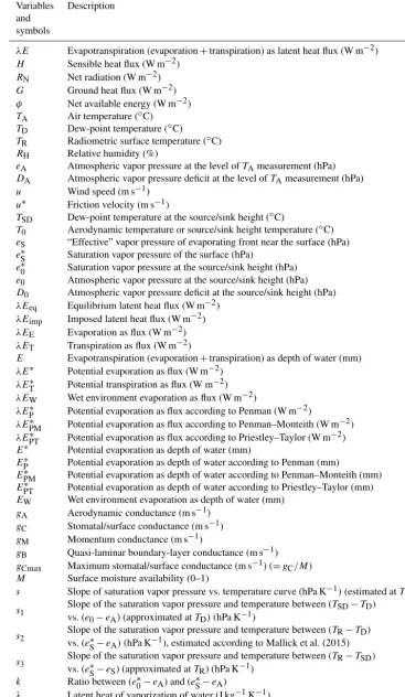
The foundation of the development of STIC is based on the goal of finding an analytical solution of the two unobserved “state variables” (gA andgC) in the PM equation while ex-ploiting the radiative (RNandG), meteorological (TA,RH), and radiometric surface temperature (TR) as external inputs. The fundamental assumption in STIC is the first-order de-pendence ofgAandgCon the aerodynamic temperature (T0) and soil moisture (throughTR). This assumption allows a di-rect integration ofTRinto the PM equation while simultane-ously constraining the conductances through TR. Although theTRsignal is implicit inRN, which appears in the numer-ator of the PM equation (Eq. 1), it may be noted thatRNhas a relatively weak dependence on TR (compared to the sen-sitivity of TR to soil moisture andλE). Given thatTR is a direct signature of the soil moisture availability, inclusion of TRin the PM equation also works to add water-stress con-trols ingC. Until now the explicit use ofTRin the PM model was hindered due to the unavailability of any direct method to integrateTRinto this model, and, furthermore, due to the lack of physical models expressing biophysical states of veg-etation as a function of TR. Therefore, the majority of the PM-basedλEmodeling approaches strongly rely on surface reflectance and meteorology while exploiting the empirical leaf-scale parameterizations of the biophysical conductances (Prihodko et al., 2008; Bonan et al., 2014; Ershadi et al., 2015).

The PM equation is commonly expressed as

λE=sφ+ρ cPgADA s+γ1+gA

gC

, (1)

whereρis the air density (kg m−3),cP is the specific heat of air (J kg−1K−1),γ is the psychrometric constant (hPa K−1), sis the slope of the saturation vapor pressure vs. air tempera-ture (hPa K−1),DAis the saturation deficit of the air (hPa) or

vapor pressure deficit at the reference level, andφis the net available energy (W m−2) (the difference between RN and G). The units of all the surface fluxes and conductances are in W m−2 and m s−1, respectively. For a dense canopy,gC in the PM equation represents the canopy surface conduc-tance. Although it is not equal to the canopy stomatal con-ductance, it contains integrated information on the stomata. For a heterogeneous landscape,gCin the PM equation is an aggregated surface conductance containing information on both canopy and soil. Traditionally, the two unknown “state variables” in Eq. (1) aregAandgC, and the STIC methodol-ogy is based on formulating “state equations” for these con-ductances that satisfy the PM model (Mallick et al., 2014, 2015). The PM equation is “closed” upon the availability of canopy-scale measurements of the two unobserved biophys-ical conductances, and if we assume the empirbiophys-ical models of gA andgC to be reliable. However, neithergA nor gC can be measured at the canopy scale or at larger spatial scales. Furthermore, as shown by some recent studies (Matheny et al., 2014; Van Dijk et al., 2015), a more appropriategA and gCmodel is currently not available. This implies that a true “closure” of the PM equation is only possible through an an-alytical estimation of the conductances.

2.2 State equations

By integrating TR with standard surface energy bal-ance (SEB) theory and vegetation biophysical principles, STIC formulates multiple “state equations” that eliminate the need for exogenous parametric submodels forgAandgC, as-sociated aerodynamic variables, and land–atmosphere cou-pling. The state equations of STIC are as follows and their detailed derivations are described in Appendix A1.

gA=

φ

ρcP

h

(T0−TA)+

e0−eA

γ

i (2)

gC=gA

(e0−eA) e∗₀−e0

(3)

T0=TA+

_e

0−eA γ

1−3 3

(4)

3= 2αs

2s+2γ+γgA

gC(1+M)

(5)

explained in Appendix A2). Given values of RN, G, TA, and RH or eA, the four state equations (Eqs. 2–5) can be solved simultaneously to derive analytical solutions for the four state variables. This also produces a “closure” of the PM model, which is independent of empirical parameteri-zations for both gA and gC. However, the analytical solu-tions to the above state equasolu-tions have four accompanying unknowns,M(surface moisture availability),e0(vapor pres-sure at the source/sink height),e₀∗(saturation vapor pressure at the source/sink height), and the Priestley–Taylor coeffi-cient (α), and as a result there are four equations with eight unknowns. Consequently an iterative solution is needed to determine the four unknown variables (as described in Ap-pendix A2), which is a further modification of the STIC1.1 framework (Mallick et al., 2015). The present version of STIC is designated as STIC1.2 and its uniqueness is the physical integration of TRinto a combined structure of the PM and Shuttleworth–Wallace (SW, hereafter) (Shuttleworth and Wallace, 1985) models to estimate the source/sink height vapor pressures (Appendix A2). In addition to physically in-tegrating TRobservations into a combined PM–SW frame-work, STIC1.2 also establishes a feedback loop describing the relationship betweenTRandλE, coupled with canopy– atmosphere components relating λE to T0 and e0. To es-timate M, the radiometric surface temperature (TR) is ex-tensively used in a physical retrieval framework, thus treat-ingTRas an external input. In Eq. (5), the Priestley–Taylor coefficient (α) appeared due to the use of the advection– aridity (AA) hypothesis (Brutsaert and Stricker, 1979) for deriving the state equation of3(Supplement S1). However, instead of optimizingαas a “fixed parameter”, we have de-veloped a physical equation ofα(Eq. A15) and numerically estimated αas a “variable”. The derivation of the equation forαis described in Appendix A2. The fundamental differ-ences between STIC1.2 and earlier versions are described in Table A1.

In STIC1.2,T0 is a function ofTR, and they are not as-sumed equal (T06=TR). The analytical expression of T0 is dependent onMand the estimation ofMis based onTR. To further elaborate this point on the inequality ofT0 andTR, we show an intercomparison of retrievedT0vs.TRfor forest and pasture (Fig. A2). This indicates the distinct difference of the retrievedT0fromTRfor the two different biomes. 2.3 PartitioningλE

The terrestrial latent heat flux is an aggregate of both transpi-ration (λET) and evaporation (λEE) (sum of soil evaporation and interception evaporation from the canopy). During rain events the land surface becomes wet and λE tends to ap-proach the potential evaporation (λE∗), while surface drying after rainfall causesλE to approach the potential transpira-tion rate (λE_T∗) in the presence of vegetation, or zero with-out any vegetation. Hence, λE at any time is a mixture of these two end-member conditions depending on the degree

of surface moisture availability or wetness (M) (Bosveld and Bouten, 2003; Loescher et al., 2005). Considering the gen-eral case of evaporation from an unsaturated surface at a rate less than the potential,Mis the ratio of the actual to potential evaporation rate and is considered as an index of evaporation efficiency during a given time interval (Boulet et al., 2015). Partitioning ofλEintoλEEandλETwas performed accord-ing to Mallick et al. (2014) as follows:

λE=λEE+λET=MλE∗+(1−M)λET∗. (6) The estimates ofλEEin the current method consist of an ag-gregated contribution from both interception and soil evap-oration, and no further attempt is made to separate these two components. In the Amazon forest, soil evaporation has a negligible contribution, while the interception evaporation contributes substantially to the total evaporative fluxes, and therefore the partitioning ofλE into λEE andλET is cru-cial. After estimatinggA,λE∗was estimated according to the Penman equation (Penman, 1948) andλETwas estimated as the residual in Eq. (6).

In this study, we use the term “canopy conductance” in-stead of “stomatal conductance” given that the term “stom-ata” is applicable at the leaf scale only. As stated earlier, for a heterogeneous surface,gCshould principally be a mixture of the canopy surface (integrated stomatal information) and soil conductances. However, given the high vegetation density of the Amazon Basin, the soil surface exposure is negligible, and hence we assumegCto be the canopy-scale aggregate of the stomatal conductance. Similarly, a differentgAexists for soil–canopy, sun–shade, and dry–wet conditions (Leun-ing, 1995), which are currently integrated into a lumpedgA (given the big-leaf nature of STIC). From the big-leaf per-spective, it is generally assumed that the aerodynamic con-ductance of water vapor and heat are equal (Raupach, 1998). However, to obtain partitioned aerodynamic conductances, explicit partitioning ofλE is needed, which is beyond the scope of the current paper.

2.4 EvaluatinggAandgC

Due to the lack of direct canopy-scalegA measurements, a rigorous evaluation ofgAcannot be performed. To evaluate the STIC retrievals ofgA(gA-STIC), we adopted three differ-ent methods.

a. By using the measured friction velocity (u∗) and wind speed (u) at the EC towers and using the equation of Baldocchi and Ma (2013) (gA-BM13) in which gA was expressed as the sum of turbulent conductance and canopy (quasi-laminar) boundary-layer conductance as gA-BM13=

h

u/u∗2+2/ ku∗2(Sc/Pr)0.67i −1

ratio is generally considered to be unity. Here the con-ductances of momentum, sensible, and latent heat fluxes are assumed to be identical (Raupach, 1998).

b. By invertingλEobservations for wet conditions, hence assumingλE∼=λE∗and estimatinggA(gA-INV) as gA-INV=γ λE/ρcPDA. (8) c. By inverting the aerodynamic equation of H and es-timating a hybrid gA (gA-HYB) from observed H and STICT0as (T0-STIC),

gA-HYB=H /ρcP(T0-STIC−TA) . (9) Like gA-STIC, direct verification of STIC gC(gC-STIC) could not be performed, as canopy-scale gC observa-tions are not possible with current measurement tech-niques. Although leaf-scalegCmeasurements are rela-tively straightforward, these values are not comparable to values retrieved at the canopy scale. However, assum-ing u∗-basedgA as the baseline aerodynamic conduc-tance, we have estimated canopy-scalegCby inverting the PM equation (gC-INV) (Monteith, 1995) to evaluate gC-STIC by exploitinggA-BM13 in conjunction with the available φ,λE,TA, and DA measurements from the EC towers.

2.5 Decoupling coefficient and biophysical controls The decoupling coefficient or “Omega” () is a dimension-less coefficient ranging from 0.0 to 1.0 (Jarvis and Mc-Naughton, 1986) and is considered as an index of the degree of stomatal control on transpiration relative to the environ-ment. The equation ofis as follows:

= s γ+1 s γ +1+

gA

gC

. (10)

Introducinginto the Penman–Monteith (PM) equation for λEresults in

λE=λEeq+(1−)λEimp, (11)

λEeq= sφ

s+γ, (12)

λEimp= ρcP

γ gCDA, (13)

whereλEeqis the equilibrium latent heat flux, which depends only onφ and would be obtained over an extensive surface of uniform moisture availability (Jarvis and McNaughton, 1986; Kumagai et al., 2004). λEimp is the imposed latent heat flux, which is “imposed” by the atmosphere on the veg-etation surface through the effects of vapor pressure deficit (triggered under limited soil moisture availability), andλE becomes proportional togC.

When thegC/gAratio is very small (i.e., water-stress con-ditions), stomata principally control the water loss, and a change ingCwill result in a nearly proportional change in transpiration. Such conditions trigger a strong biophysical control on transpiration. In this case thevalue approaches zero and vegetation is believed to be fully coupled to the at-mosphere. In contrast, for a highgC/gAratio (i.e., high water availability), changes ingCwill have little effect on the tran-spiration rate, and trantran-spiration is predominantly controlled byφ. In this case thevalue approaches unity, and vegeta-tion is considered to be poorly coupled to the atmosphere.

Given that bothgAandgCare the independent estimates in STIC1.2, the concept ofwas used to understand the degree of biophysical control onλET, which indicates the extent to which the transpiration fluxes are approaching the equilib-rium limit. However, the biophysical characterization ofλET andλEEthrough STIC1.2 significantly differs from previous approaches (Ma et al., 2015; Chen et al., 2011; Kumagai et al., 2004), and the fundamental differences are centered on the specifications ofgA andgC(as described in Table A2). While the estimation ofgAin previous approaches was based onuandu∗, the estimation ofgCwas based on inversion of observedλE based on the PM equation (e.g., Stella et al., 2013). However, none of these approaches allow indepen-dent quantification of biophysical controls of λE, as gC is constrained byλEitself.

3 Datasets

Eddy covariance and meteorological quantities

We used the LBA (Large-Scale Biosphere-Atmosphere Ex-periment in Amazonia) data for quantifying the biophysical controls on the evaporative flux components. LBA was an in-ternational research initiative conducted during 1995–2005 to study how Amazonia functions as a regional entity within the larger Earth system, and how changes in land use and cli-mate will affect the hydrological and biogeochemical func-tioning of the Amazon ecosystem (Andreae et al., 2002).

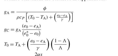
Table 2.Overview of the LBA tower sites. Here, (–) refers to (S) and (W) for latitude and longitude, respectively.

Biome PFT Site LBA Data Latitude Longitude Tower Annual code availability (◦) (◦) height rainfall

period (m) (mm)

Forest Tropical Manaus K34 Jun 1999 to −2.609 −60.209 50 2329 rainforest KM34 Sep 2006

(TRF)

Forest Tropical Santarem K67 Jan 2002 to −2.857 −54.959 63 1597 moist KM67 Jan 2006

forest (TMF)

Forest Tropical Santarem K83 Jul 2000 to −3.018 −54.971 64 1656 moist KM83 Dec 2004

forest (TMF)

Forest Tropical Reserva RJA Mar 1999 to −10.083 −61.931 60 2354 dry forest Biológica Oct 2002

(TDF) Jarú

Pasture Pasture Santarem K77 Jan 2000 to −3.012 −54.536 18 1597 (PAS) KM77 Dec 2001

Pasture Pasture Fazenda FNS Mar 1999 to −10.762 −62.357 8.5 1743 (PAS) Nossa Oct 2002

Senhora

adopted by Anderson et al. (2007) and Mallick et al. (2015). In the absence of G measurements, φ was assumed to be equal to the sum of λE andH with the assumption that a dense vegetation canopy restricts the energy incident on the soil surface, thereby allowing us to assume negligible ground heat flux. For the present analysis, data from six selected EC towers (Table 2) represent two different biomes (forest and pasture) covering four different PFTs, namely, tropical rainforest (TRF), tropical moist forest (TMF), tropical dry forest (TDF), and pasture (PAS), respectively. A general de-scription of the datasets can be found in Saleska et al. (2013). For all sites, monthly averages of the diurnal cycle (hourly time resolution) were chosen for the present analysis.

4 Results

4.1 EvaluatinggA,gC, and surface energy balance

fluxes

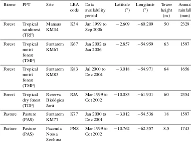
Examples of monthly averages of the diurnal cycles of the four differentgA estimates and their correspondinggC esti-mates over two different PFTs (K34 for forest and FNS for pasture) reveal thatgA-STICandgC-STICtend to be generally higher for the forest than their counterparts, varying from 0 to 0.06 m s−1and 0 to 0.04 m s−1respectively (Fig. 1a and b). The magnitude ofgA-STICvaried between 0 and 0.025 m s−1 for the pasture (Fig. 1a), while gC-STIC values were less

than half of those estimated over the forest (0–0.01 m s−1) (Fig. 1b). The conductances showed a marked diurnal vari-ation expressing their overall dependence on net radivari-ation, vapor pressure deficit, and surface temperature. Despite the absolute differences between the conductances from the dif-ferent retrieval methods, their diurnal patterns were compa-rable.

relation-(a)Time series gA

(b)Time series gC

Jan Feb Mar Apr May Jun Jul Aug Sep Oct Nov Dec

0 0.02 0.04 0.06 0.08

Month

gA

(m

s

-1 )

Forest

Jan Feb Mar Apr May Jun Jul Aug Sep Oct Nov Dec

0 0.02 0.04 0.06 0.08

Month

gA

(m

s

-1 )

Pasture gA-STIC

g

A-BM13

g

A-INV

g

A-HYB

Jan Feb Mar Apr May Jun Jul Aug Sep Oct Nov Dec 0

0.02 0.04 0.06

Month

g C

(m

s

-1 )

Forest

Jan Feb Mar Apr May Jun Jul Aug Sep Oct Nov Dec 0

0.02 0.04 0.06

Month

g C

(m

s

-1 )

Pasture gC-STIC

g_C-g A-BM13 g_C-g

A-INV g_C-g

A-HYB

Figure 1.Examples of monthly averages of the diurnal time series of canopy-scale(a)gAand(b)gCestimated for two different biomes (forest and pasture) in the Amazon Basin (LBA sites K34 and FNS). The time series of four differentgAestimates and their corresponding gCestimates are shown here.

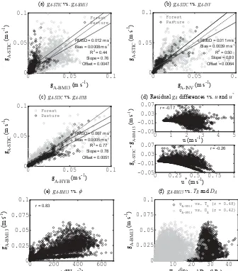
ship between the residualgAdifference with either u∗or u (r= −0.26 and−0.17). However, a considerable relationship was found between wind- and shear-drivengA(i.e.,gA-BM13) vs.φ,TR, andDA(r=0.83, 0.48, and 0.42) (Fig. 2e and f), which indicates that these three energy and water constraints can explain 69, 23, and 17 % variance of gA-BM13, respec-tively.

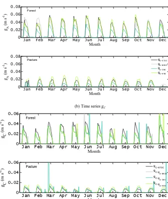
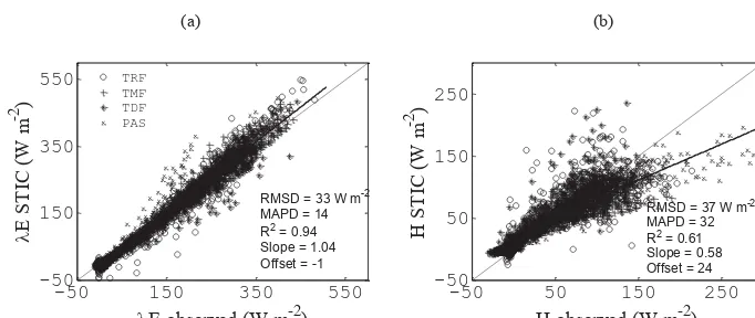
Canopy-scale evaluation of hourly gC is presented in Fig. 3a (and Table 3), combining data from the four PFTs. Estimated values range between zero and 0.06 m s−1 for gC-STIC and show reasonable correlation (R2=0.39) (R2 range between 0.14 [±0.04] and 0.58 [±0.12]) between gC-STIC andgC-INV, with regression parameters ranging be-tween 0.30 (±0.022) and 0.85 (±0.025) for the slope and between 0.0024 (±0.0003) and 0.0097 (±0.0007) m s−1for

the offset (Table 3). The RMSD varied between 0.007 (PAS) and 0.012 m s−1(TRF and TDF). Given thatgAsignificantly controls gC, we also examined whether biases in gC are introduced by ignoring wind and shear information within STIC. The scatter plots between the residualgC difference (gC-STIC−gC-INV) vs. both u andu∗ (Fig. 3b) showed gC residuals to be evenly distributed across the entire range ofu andu∗, and no systematic pattern was evident.

DgA-STICYVgA-BM13 EgA-STICYVgA-INV

FgA-STICYVgA-HYB G5HVLGXDOgAGLIIHUHQFHVYVuDQGu

*

HgA-BM13YVI IgA-BM13YVTRDQGDA

0 0.05 0.1

0 0.05 0.1

J_$%0PV

J$

67

,&

P

V

506' PV

%LDV PV

5

Slope = 0.76 Offset = 0.0047

Forest Pasture

0 0.05 0.1

0 0.05 0.1

J_$,19PV

J$

67

,&

P

V

506' PV

%LDV PV

5

Slope = 0.80 Offset = 0.0064

Forest Pasture

0 0.05 0.1

0 0.05 0.1

J_$+<%PV

J$

67

,&

P

V

506' PV

%LDV PV

5

Slope = 0.78 Offset = 0.0051

Forest Pasture

0 1 2 3 4 5

-0.05 -0.01 0.03 0.07

XPV

U

0 0.25 0.5 0.75 1

-0.05 -0.01 0.03 0.07

XPV J$

6

7

,&

J$

%

0

P

V

U

0 200 400 600

0 0.025 0.05 0.075 0.1

I:P

J $

%

0

P

V

U

10 20 30 40

0 0.025 0.05 0.075 0.1

7₅&DQG'_$K3D

J $

%

0

P

V

g_A-BM13 vs. T_R (r = 0.48) g

A-BM13 vs. DA (r = 0.42)

Figure 2. (a)Comparison between STIC-derivedgA(gA-STIC) with an estimated aerodynamic conductance based on friction velocity (u∗) and wind speed (u) according to Baldocchi and Ma (2013) (gA-BM13),(b) comparison betweengA-STIC with an invertedgA (gA-INV) based on EC observations ofλEandDA,(c)comparison betweengA-STICwith a hybridgA(gA-HYB)based on EC observations ofH and estimatedT0over the LBA EC sites,(d)comparison between residualgAdifferences vs.uandu∗, and(e, f)relationship between wind- and shear-derivedgAvs.φ,TR, andDAover the LBA EC sites.

(Fig. 4), respectively. Regression parameters varied between 0.96 (±0.008) and 1.14 (±0.010) for the slope and be-tween −16 (±2) and −2 (±2) W m−2 for the offset for λE (Table 4), whereas forH, these were 0.60 (±0.025) to 0.89 (±0.035) for the slope and 9 (±1) to 29 (±2) W m−2 for the offset (Table 3), respectively. The RMSD inλEvaried from 20 to 31 W m−2and from 23 to 34 W m−2forH (Ta-ble 3).

The evaluation of the conductances and surface energy fluxes indicates some efficacy for the STIC-derived fluxes and conductance estimates that represent a weighted average of these variables over the source area around the EC tower.

(a)Tower scale evaluation of gC (b)Residual gC differences vs. u and u*

0 0.02 0.04 0.06 0.08

0 0.02 0.04 0.06 0.08

g

C-INV (m s -1

)

g C

-S

T

IC

(m

s

-1 )

RMSD = 0.010 m s-1

Bias = -0.0006 m s-1

R2 _{= 0.39}

slope = 0.64 offset = 0.0045

Forest Pasture

0 1 2 3 4 5

-0.05 -0.01 0.03 0.07

u (m s-1)

g C

-S

T

IC

g C

-IN

V

(

m

s

-1)

0 0.25 0.5 0.75 1

-0.05 -0.01 0.03 0.07

u* (m s-1)

Figure 3. (a)Comparison between STIC-derivedgC(gC-STIC) andgCcomputed by inverting the PM model (gC-INV) over the LBA EC sites, wheregA-BM13was used as aerodynamic input in conjunction with tower measurements ofλE, radiation and meteorological variables, and(b)residualgCdifferences vs. wind speed (u) and friction velocity (u∗) over the LBA EC sites.

(a) (b)

-50 150 350 550

-50 150 350 550

O

E

ST

IC

(W

m

-2 )

OE observed (W m-2) RMSD = 33 W m-2

MAPD = 14 R2 _{= 0.94}

Slope = 1.04 Offset = -1

TRF TMF TDF PAS

-50 50 150 250

-50 50 150 250

H

ST

IC

(W

m

-2 )

H observed (W m-2) RMSD = 37 W m-2

MAPD = 32 R2 _{= 0.61}

Slope = 0.58 Offset = 24

Figure 4.Comparison between STIC-derived(a)λEand(b)H over four different PFTs in the Amazon Basin (LBA tower sites). MAPD is the percent error defined as the mean absolute deviation between the predicted and observed variables divided by the mean observed variable.

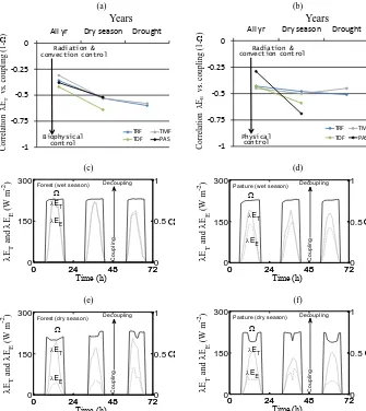
(r= −0.29 to−0.45) between (1−) andλEE(Fig. 5b) in all four PFTs indicated the role of aerodynamic control on λEE. The aerodynamic control was also enhanced during the dry seasons, as shown by the increased negative correlation (r= −0.50 to−0.69) (Fig. 5b) between (1−) andλEE.

Illustrative examples of the diurnal variations of λEE, λET, and  for two different PFTs with different annual rainfall (2329 mm in rainforest, K34, and 1597 mm in pas-ture, FNS) for 3 consecutive days during both dry and wet seasons are shown in Fig. 5c–f. This shows the morning rise ofand a near-constant afternoonin the wet season (Fig. 5c and 5d), thus indicating no biophysical controls on λEEandλETduring this season. By contrast, during the dry season, the morning rise inis followed by a decrease dur-ing noontime (15 to 25 % increase in coupldur-ing in forest and pasture) (Fig. 5e and f) due to dominant biophysical control, which is further accompanied by a transient increase from mid-afternoon till late afternoon, and steadily declines there-after. Interestingly, coupling was relatively higher in pasture during the dry seasons, and the reasons are detailed in the following section and discussion.

4.3 gCandgAvs. transpiration and evaporation

(a) (b)

(c) (d)

(e) (f)

-1 -0.75 -0.5 -0.25 0

All yr Dry season Drought

Corre lation  ET vs. coupling (1 - ) Years TRF TMF TDF PAS Biophysical control Radiation & convection control -1 -0.75 -0.5 -0.25 0

All yr Dry season Drought

Corre lation  EE vs. coupling (1 - ) Years TRF TMF TDF PAS Physical control Radiation & convection control

0 24 48 72

0 150 300 Time (h)  ET an d  EE (W m

-2 ) _

E

E

E_T

C ou pl in g Decoupling Forest (wet season)

0 24 48 720

0.5 1



0 24 48 72

0 150 300 Time (h)  ET an d  EE (W m -2 ) E T  E E Co up lin g Decoupling Pasture (wet season)

0 24 48 720

0.5 1



0 24 48 72

0 150 300 Time (h)  ET an d  EE (W m -2 ) 

E_E

E_T

Co

up

lin

g

Decoupling Forest (dry season)

0 24 48 720

0.5 1



0 24 48 72

0 150 300 Time (h)  ET an d  EE (W m -2 )

E_T 

E_E

C ou pl in g Decoupling Pasture (dry season)

0 24 48 720

0.5 1



Figure 5.Correlation of coupling (1−) with(a)transpiration (λET)and(b)evaporation (λEE) and over four different PFTs by combining data for all the years, only during dry seasons for all the years, and during drought year 2005. Data for 2005 were not available for TDF and PAS.(c)–(e)Examples of the diurnal pattern of(black lines),λEE(grey dotted lines) andλET(grey solid lines) estimated over two ecohydrologically contrasting biomes (K34 for forest and FNS for pasture) in the Amazon Basin (LBA tower sites) during wet and dry seasons.

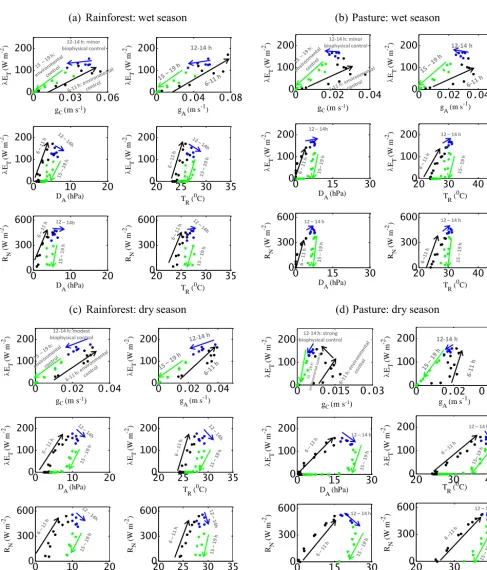
changes inRN(15 to 50 % change),DA(20 to 60 % change), andTR (5 to 14 % change), which indicates the absence of any dominant biophysical regulation onλETduring the wet season (Fig. 7a and b). On the contrary, in the dry season, al-though the morning rise inλETis steadily controlled by the integrated influence of environmental variables, a modest to strong biophysical control is found for both PFTs during the afternoon, whereλETsubstantially decreased with decreas-ing conductances (Fig. 7c and d). This decrease in λET is mainly caused by the reduction ingCas a result of increas-ingDAandTR(as seen later in Fig. 8a and c). In the dry sea-son, the area under the hysteretic relationship betweenλET, gC, and environmental variables was substantially wider in pasture (Fig. 7d) than for the rainforest (Fig. 7c), which is attributed to a greater hysteresis area between RN andDA in pasture as a result of reduced water supply. The stronger

hysteresis effects in pasture during the dry season (Fig. 7d) ultimately led to the stronger relationship between coupling andλET(as seen in Fig. 5a).

4.4 Factors affecting variability ofgCandgA

(a)ET versus gC (b) EE versus gC

(c) ET versus gA (d)EE versus gA

0 0.02 0.04 0.06 0.08

0 100 200 300



E T

(W

m

-2 )

g C (m s

-1 )

TRF TMF TDF PAS

0 0.02 0.04 0.06 0.08

0 100 200 300



E E

(W

m

-2 )

g C (m s

-1 )

0 0.025 0.05 0.075 0.1

0 100 200 300



E T

(W

m

-2 )

g A (m s

-1₎

0 0.025 0.05 0.075 0.1

0 100 200 300



E E

(W

m

-2 )

g A (m s

-1 )

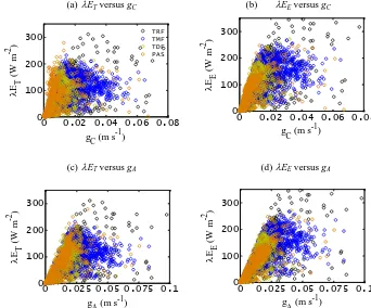
Figure 6.Scatter plots of transpiration (λET) and evaporation (λEE) vs.gCandgAover four different PFTs in the Amazon Basin (LBA tower sites).

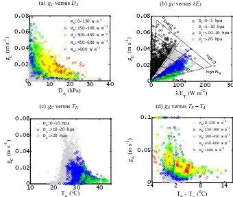
the data withr values of 0.38 (0< RN<150 W m−2), 0.63 (150< RN<300 W m−2), 0.73 (300< RN<450 W m−2), 0.78 (450< RN<600 W m−2), and 0.87 (RN>600 W m−2). The sensitivity of gC to DA was at the maximum in the high RN range beyond 600 W m−2 and the sensitivity pro-gressively declined with declining magnitude of RN (0– 150 W m−2).

Scatter plots between gC and λET for different levels of DA revealed a linear pattern between them for a wide range of DA (20> DA>0 hPa) (Fig. 8b). Following Mon-teith (1995), isopleths ofRNare delineated by the solid lines passing through λET on thex axis and through gC on the y axis. Isobars ofDA (dotted lines) pass through the origin because λET approaches zero as gC approaches zero. Fig-ure 8b shows substantial reduction ofgCwith increasingDA without any increase inλET, like an inverse hyperbolic pat-tern toDA(Monteith, 1995; Jones, 1998). For all the PFTs, an active biological (i.e., stomatal) regulation maintained al-most constantλETwhenDAwas changed from low to high values (Fig. 8b). At highDA(above 10 hPa), after an initial increase in λETwithgC,gC approached a maximum limit and remained nearly independent ofλET(Fig. 8b). Among all theDAlevels, the maximum control ofgConλET vari-ability (62 to 80 %) was found at high atmospheric water demand (i.e., 30 hPa> DA>20 hPa). The scatter plots be-tween gC and TR (Fig. 8c) for different levels of DA

re-vealed an exponential decline ingCwith increasingTR and atmospheric water demand. When retrievedgA was plotted against the radiometric surface temperature and air tempera-ture difference (TR−TA), an exponential decline ingAwas found in response to increasing (TR−TA) (Fig. 8d). High gAis persistent with low (TR−TA) irrespective of the varia-tions inRN(with the exception of very lowRN). Four nega-tively logarithmic scatters fit thegA vs. (TR−TA) relation-ship withr values of 0.28 (150< RN<300 W m−2), 0.55 (3000< RN<450 W m−2), 0.64 (450< RN<600 W m−2), and 0.77 (RN>600 W m−2).

5 Discussion

5.1 EvaluatinggA,gC, and surface energy balance

fluxes

(a)

Rainforest: wet season

(b)

Pasture: wet season

(c) Rainforest: dry season

(d) Pasture: dry season

0 0.03 0.06

0 100 200  ET (W m -2) g

S (m s

-1

)

0 0.04 0.08

0 100 200  ET (W m -2 ) g

A (m s

-1

)

0 10 20

0 100 200  ET (W m -2) D

A (hPa)

20 25 30 35

0 100 200  ET (W m -2 ) T

R ( 0

C)

0 10 20

0 300 600 RN (W m -2) D

A (hPa)

20 25 30 35

0 300 600

T

R ( 0 C) RN (W m -2 ) 12-14 h 12-14 h: minor

biophysical control

gC (m s-1)

0 0.02 0.04

0 100 200 E T (W m -2 ) g

S (m s

-1

)

0 0.02 0.04

0 100 200 E T (W m -2 ) g

A (m s

-1

)

0 15 30

0 100 200 E T (W m -2 ) D

A (hPa)

20 30 40

0 100 200 E T (W m -2 ) T

R ( 0

C)

0 15 30

0 300 600 RN (W m -2 )

D_A (hPa)

20 30 40

0 300 600

T

R ( 0 C) RN (W m -2 )

12 – 14 h 12-14 h

12 – 14h

12-14 h: minor biophysical control

12 – 14 h 12 – 14 h

gC (m s-1)

0 0.02 0.04

0 100 200  ET (W m -2 )

g_S (m s-1)

0 0.02 0.04

0 100 200  ET (W m -2 )

g_A (m s-1)

0 10 20

0 100 200  ET (W m -2 ) D

A (hPa)

20 25 30 35

0 100 200  ET (W m -2 )

T_R (0C)

0 10 20

0 300 600 RN (W m -2 ) D

A (hPa)

20 25 30 35

0 300 600

T_R (0C)

RN

(W

m

-2 ) 12-14 h: modest

biophysical control

gC (m s-1)

0 0.015 0.03

0 100 200 E T (W m -2 ) g

C (m s

-1

)

0 0.02 0.04

0 100 200 E T (W m -2 ) g

A (m s

-1

)

0 15 30

0 100 200 E T (W m -2 ) D

A (hPa)

20 30 40

0 100 200 E T (W m -2 ) T

R ( 0

C)

0 15 30

0 300 600 RN (W m -2 ) D

A (hPa)

20 30 40

0 300 600

T

R ( 0 C) RN (W m -2 )

12 – 14 h 12-14 h

12 – 14 h 12-14 h: strong biophysical control

12 – 14 h 12 – 14 h

gC (m s-1)

(a)gC versus DA (b)gC versus ET

(c)gC versus TR (d)gA versus TR – TA

0 10 20 30 40

0 0.02 0.04 0.06 0.08

D_A (hPa)

g C

(m

s

-1 )

R_N:0-150 W m-2

RN:150-300 W m -2

R_N:300-450 W m-2

R_N:450-600 W m-2

R_N:>600 W m-2

0 100 200 300

0 0.02 0.04 0.06 0.08

E_T (W m-2)

gC

(m

s

-1 )

low _D

A

hig h D

A

low R_N

high R

N

D_A:0-5 hpa DA:5-10 hpa

D_A:>10-20 hpa D_A:>20 hpa

10 20 30 40

0 0.02 0.04 0.06 0.08

T_R (°C)

g C

(m

s

-1 )

D_A:0-10 hpa DA:>10-20 hpa

D_A:>20 hpa

-40 2 8 14

0.05 0.1

T_R - T_A (0C)

g A

(m

s

-1 )

R

N:0-150 W m -2

R

N:150-300 W m -2

R_N:300-450 W m-2

R

N:450-600 W m -2

R

N:>600 W m -2

Figure 8. (a)Response of retrievedgCto atmospheric vapor pressure deficit (DA) for different classes of net radiation (RN),(b)response of retrievedgCto transpiration for different classes ofDA,(c)response of retrievedgCto radiometric surface temperature (TR) for different classesDA, and(d)relationship between retrievedgAand radiometric surface temperature and air temperature difference (TR−TA) in the Amazon Basin (LBA tower sites).

((2/ku∗2)(Sc/Pr)0.67) ingA-BM13, which results in some dis-crepancies betweengA-STICandgA-BM13, particularly in the pasture (Fig. 2a). The extent to which the structural discrep-ancies between gA-STIC andgA-BM13 relate to actual differ-ences in the conductances for momentum vs. heat is be-yond the scope of this paper, and a detailed investigation using data on atmospheric profiles of wind speed, temper-ature, etc. are needed to actually quantify such differences. Momentum transfer is associated with pressure forces and is not identical to heat and mass transfer (Massman, 1999). In STIC1.2,gAis directly estimated and is a robust representa-tive of the conductances to heat (and water vapor) transfer, whereasgA-BM13estimates based onu∗anduare more rep-resentative of the momentum transfer. Therefore, the differ-ence between the two differentgA estimates (Fig. 2) can be largely attributed to the actual difference in the conductances for momentum and heat (water vapor). The turbulent con-ductance equation (u∗2/u) ingA-BM13is also very sensitive to the uncertainties in the sonic anemometer measurement (Contini et al., 2006; Richiardone et al., 2012). However, the evidence of a weak systematic relationship between thegA residuals and u (Fig. 2d) and the capability of the thermal (TR), radiative (φ), and meteorological (TA,DA)variables in capturing the variability ofgA-BM13 (Fig. 2e and f)

re-(a)D0 vs. DA over four PFTs (b)Distribution of gC/gA ratio over four PFTs

(c)gC/gA vs. TR-TA over four PFTs

0 10 20 30 40

0 10 20 30 40

D_A (hPa) D0 ( hP a) TRF Unco upling( equilibr ium) Coupl ing(im

posed)

gC/gA<0.5 g_C/g_A>0.5

0 10 20 30 40

0 10 20 30 40

D_A (hPa) D0 ( hP a) TMF Unco upling( equilibr ium) Coupl ing(im

posed)

gC/gA<0.5 g_C/g_A>0.5

0 10 20 30 40

0 10 20 30 40

D_A (hPa) D0 ( hP a) TDF Unco upling( equilibr ium) Coupl ing(im

posed)

gC/gA<0.5 g_C/g_A>0.5

0 10 20 30 40

0 10 20 30 40

D_A (hPa) D0 ( hP a) PAS Unco upling( equilibr ium) Coupl ing(im pose d)

gC/gA<0.5 g_C/g_A>0.5

0 0.5 1

0 300 600 _TRF Biophysical control Radiation control

g_C/g_A ratio

F

re

que

nc

y

0 0.5 1

0 500 1000 1500 _TMF Biophysical control Radiation control

g_C/g_A ratio

F

re

que

nc

y

0 0.5 1

0 250 500 TDF Biophysical control Radiation control

g_C/g_A ratio

F

re

que

nc

y

0 0.5 1

0 250 500 PAS Biophysical control Radiation control

g_C/g_A ratio

F

re

que

nc

y

0 5 10 15

0 0.5 1

g C /g A

T_R - T_A(0C) Dry seas_on Wet season TRF TMF TDF PAS

Figure 9. (a)Scatter plots between source/sink height (or in-canopy) vapor pressure deficit (D0) and atmospheric vapor pressure deficit (DA) for two different classes ofgC/gAratios over four PFTs, which clearly depicts a strong coupling betweenD0andDAfor lowgC/gAratios.

(b)Histogram distribution ofgC/gAratios over the four PFTs in the Amazon Basin (LBA tower sites).(c)Scatter plots betweengC/gA ratio vs. surface air temperature difference (TR−TA) for the four PFTs during the wet season and dry season in the Amazon Basin (LBA tower sites).

sults (Fig. 4), it appears thatgA-STICtends to be the appro-priate aerodynamic conductance that satisfies the PM–SW equation. Discrepancies between gC-STIC andgC-INV origi-nated from the differences ingAestimates between the two methods.

Despite the good agreement between the measured and predicted λE and H (Fig. 4, Table 4), the larger error in H was associated with the higher sensitivity ofH to the er-rors inTR(due to poor emissivity correction) (Mallick et al., 2015). Since the difference between TR andTA is consid-ered to be the primary driving force ofH(van der Tol et al., 2009), the modeled errors inH are expected to arise due to the uncertainties associated withTR.

5.2 Canopy coupling,gC, andgAvs. transpiration and

evaporation

Table 3.Comparative statistics for the STIC- and tower-derived hourlygAandgCfor a range of PFTs in the Amazon Basin (LBA tower sites). Values in parentheses are±1 standard deviation (standard error for correlation).

gA-STICvs.gA-BM13 gC-STICvs.gC-INV

PFTs RMSD R2 Slope Offset RMSD R2 Slope Offset N (m s−1) (m s−1) (m s−1) (m s−1)

TRF 0.013 0.41 1.07 0.0031 0.012 0.14 0.39 0.0097 1159 (±0.03) (±0.047) (±0.0008) (±0.04) (±0.039) (±0.0007)

TMF 0.012 0.55 0.81 0.0006 0.009 0.55 0.85 0.0032 1927 (±0.12) (±0.023) (±0.0006) (±0.12) (±0.025) (±0.0005)

TDF 0.007 0.49 0.89 0.0019 0.012 0.33 0.30 0.0050 787 (±0.15) (±0.041) (±0.0006) (±0.19) (±0.022) (±0.0005)

PAS 0.012 0.22 1.03 0.0059 0.007 0.58 0.65 0.0024 288 (±0.18) (±0.083) (±0.0007) (±0.12) (±0.025) (±0.0003)

Mean 0.012 0.44 0.76 0.0047 0.010 0.39 0.63 0.0046 4161

(±0.10) (±0.016) (±0.003) (±0.08) (±0.016) (±0.0003)

N: number of data points; RMSD: root mean square deviation between predicted (P) and observed (O) variables=

" 1 N

N P

i=0

Pi−Oi2

#2

.

Table 4.Comparative statistics for the STIC- and tower-derived hourlyλEandH for a range of PFTs in the Amazon Basin (LBA tower sites). Values in parentheses are±1 standard deviation (standard error for correlation).

λE H

PFTs RMSD R2 Slope Offset RMSD R2 Slope Offset N

(W m−2) (W m−2) (W m−2) (W m−2)

TRF 28 0.96 1.10 −16 34 0.52 0.60 29 1159

(±0.007) (±0.008) (±2) (±0.030) (±0.025) (±2)

TMF 20 0.98 1.08 −11 23 0.71 0.61 20 1927

(±0.004) (±0.004) (±1) (±0.019) (±0.014) (±1)

TDF 26 0.96 0.96 −7 30 0.66 0.89 20 787

(±0.009) (±0.008) (±2) (±0.032) (±0.035) (±3)

PAS 31 0.96 1.14 −2 33 0.88 0.67 9 288

(±0.009) (±0.010) (±2) (±0.016) (±0.011) (±1)

Mean 33 0.94 1.04 −1 37 0.61 0.58 24 4161

(±0.005) (±0.005) (±1) (±0.021) (±0.009) (±2)

canopy surface and substantially high gA compared to gC, thus resulting in lowgC/gAratios regardless of their absolute values (Meinzer et al., 1993; McNaughton and Jarvis, 1991). Here, a fractional change ingCresults in an equivalent frac-tional change inλET. This impedes transpiration from pro-moting local equilibrium ofD0and minimizing (or maximiz-ing) the gradient betweenD0and atmospheric vapor pressure deficit (DA) (i.e.,D0∼=DAorD0> DA) (Eq. A10) (Fig. 9a), thereby resulting in strong coupling between D0 and DA (Meinzer et al., 1993; Jarvis and McNaughton, 1986). Be-sides, a supplemental biophysical control onλETmight have been imposed as a consequence of a direct negative feedback

the dominance ofRN-driven equilibrium evaporation in these PFTs (Hasler and Avissar, 2007; da Rocha et al., 2009; Costa et al., 2010). In the TRF and TMF, 94 and 99 % of the re-trievedgC/gA ratios fall above 0.5, and only 1 and 6 % of the retrievedgC/gAratios fall below the 0.5 range (Fig. 9b). In contrast, 90 and 73 % of thegC/gAratios range above 0.5, and 10 to 27 % of thegC/gAratios were below 0.5 for TDF and PAS, respectively (Fig. 9b). This shows that, although ra-diation control is prevailing in all the sites, biophysical con-trol is relatively stronger in TDF and PAS as compared to the other sites. For largegC/gAratios, the conditions within the planetary boundary layer (PBL) become decoupled from the synoptic scale (McNaughton and Jarvis, 1991) and the net radiative energy becomes the important regulator of transpi-ration. For smallgC/gA ratios (e.g., in the dry season), the conditions within the PBL are strongly coupled to the atmo-sphere above by rapid entrainment of air from the capping inversion and by some ancillary effects of sensible heat flux on the entrainment (McNaughton and Jarvis, 1991). These findings substantiate the earlier theory of McNaughton and Jarvis (1991), who postulated that largegC/gAratios result in minor biophysical control on canopy transpiration due to the negative feedback on the canopy from the PBL. The neg-ative relationship between 1−andλEE(Fig. 5b) over all the PFTs is due to the feedback ofgAongC. However, over all the PFTs, a combined control of gA and environmental variables onλEEagain highlighted the impact of realistically estimatedgAonλEE(Holwerda et al., 2012).

It is important to mention that forests are generally ex-pected to be better coupled to the atmosphere as compared to the pastures, which is related to generally higher gA of the forests (due to high surface roughness). This implies that forests exhibit stronger biophysical control on λET. How-ever, due to the broad leaves of the rainforests (larger leaf area index) and higher surface wetness (due to higher rainfall amounts), the wet surface area is much larger in the forests than in the pastures. This results in much higher gCvalues for forests than for pastures during the wet season (gC≈gA), andgC/gA→1. Consequently, no significant difference in coupling was found between them during the wet season (Fig. 5c and d). Despite the absolute differences ingA and gC between forest and pasture, the high surface wetness is largely offsetting the expected difference between them. Although the surface wetness is substantially lower during the dry season, the high water availability in the forests due to the deeper root systems helps in maintaining a relatively high gC compared to the pastures. Hence, despite gA (for-est)> gA(pasture) during the dry season, substantially lower gCvalues for the pasture result in a lowergC/gAratio for the pasture compared to the forest, thus causing more biophysi-cal control onλETduring the dry season. The relatively bet-ter relationship between coupling vs.λETin PAS and TDF during the dry season was also attributed to high surface air temperature differences (TR−TA) in these PFTs that resulted in lowgC/gAratios (Fig. 9c).

5.3 Factors affectinggCandgAvariability

The stomatal feedback-response hypothesis (Monteith, 1995) also became apparent at the canopy scale (Fig. 8a and b), which states that a decrease ingC with increasing DA is caused by a direct increase inλET (Monteith, 1995; Matzner and Comstock, 2001; Streck, 2003), and gC re-sponds to the changes in the air humidity by sensingλET rather thanDA. This feedback mechanism is found because of the influence of DA on both gC and λET, which in turn changesDA by influencing the air humidity (Monteith, 1995). The change in gC is dominated by an increase in the net available energy, which is partially offset by an in-crease inλET. After the net energy input in the canopy ex-ceeds a certain threshold,gC starts decreasing even ifλET increases. HighλET increases the water potential gradient between guard cells and other epidermal cells or reduces the bulk leaf water potential, thus causing stomatal closure (Monteith, 1995; Jones, 1998; Streck, 2003). The control of soil water on transpiration also became evident from the scat-ter plots betweengCvs.λETandTRfor differentDAlevels (Figs. 8b, c, and 7). Denmead and Shaw (1962) hypothesized that reducedgCand stomatal closure occurs at moderate to higher levels of soil moisture (high λET) when the atmo-spheric demand of water vapor increases (highDA). The wa-ter content in the immediate vicinity of the plant root depletes rapidly at highDA, which decreases the hydraulic conductiv-ity of soil, and the soil is unable to efficiently supply water under these conditions. For a given evaporative demand and available energy, transpiration is determined by thegC/gA ratio, which is further modulated by the soil water availabil-ity. These combined effects tend to strengthen the biophys-ical control on transpiration (Leuzinger and Kirner, 2010; Migletta et al., 2011). The complex interaction betweengC, TR, andDA (Fig. 8c) explains why different parametricgC models produce divergent results.

AlthoughλET andλEE estimates are interdependent on gC andgA (as shown in Figs. 6–8), the figures reflect the credibility of the conductances as well as transpiration es-timates by realistically capturing the hysteretic behavior between biophysical conductances and water vapor fluxes, which is frequently observed in natural ecosystems (Zhang et al., 2014; Renner et al., 2016) (also Zuecco et al., 2016). These results are also compliant with the theories postulated earlier from observations that the magnitude of hysteresis de-pends on the radiation–vapor pressure deficit time lag, while the soil moisture availability is a key factor modulating the hysteretic transpiration–vapor pressure deficit relation as soil moisture declines (Zhang et al., 2014; O’Grady et al., 1999; Jarvis and McNaughton, 1986). This shows that despite be-ing independent of any predefined hysteretic function, the interdependent conductance–transpiration hysteresis is still captured in STIC1.2.

(i.e., high gA), a close coupling exists between the surface and the atmosphere, which causes TR and TA to converge (i.e.,TR−TA→0). WhengAis low, the difference between TRandTAincreases due to poor vertical mixing of the air.

6 Conclusions

By integrating the radiometric surface temperature (TR) into a combined structure of the PM–SW model, we have esti-mated the canopy-scale biophysical conductances and quan-tified their control on the terrestrial evapotranspiration com-ponents in a simplified SEB modeling perspective that treats the vegetation canopy as “big-leaf”. The STIC1.2 biophysi-cal modeling scheme is independent of any leaf-sbiophysi-cale empiri-cal parameterization for stomata and associated aerodynamic variables.

Stomata regulate the coupling between terrestrial carbon and water cycles, which implies that their behavior under global environmental change is critical to predicting vege-tation functioning (Medlyn et al., 2011). The combination of variability in precipitation (Hilker et al., 2014) and land cover change (Davidson et al., 2012) in the Amazon Basin is expected to increase the canopy–atmosphere coupling of pasture or forest systems under drier conditions by altering the ratio of the biological and aerodynamic conductances. An increase in biophysical control will most likely be an indica-tor of shifting the transpiration from an energy-limited to a water-limited regime (due to the impact ofTR,TA, andDA on thegC/gA ratio), with further consequences for the sur-face water balance and rainfall recycling. At the same time, a transition from forest to pasture or agriculture lands will sub-stantially reduce the contribution of interception evaporation in the Amazon; hence, it will affect the regional water cycle. This might change the moisture regime of the Amazonian Basin and affect the moisture transport to other regions. In this context, STIC1.2 provides a new quantitative and inter-nally consistent method for interpreting the biophysical con-ductances and is able to quantify their controls on the water cycle components in response to a range of climatic and eco-hydrological conditions (excluding rising atmospheric CO2) across a broad spectrum of PFTs. It could also provide the basis for improving existing land surface parameterizations for simulating vegetation water use at large spatial scales.

It should also be noted that although the case study de-scribed here provides general insights into the biophysical controls ofλEand associated feedback betweengC,DA,TR, andλET in the framework of the PM–SW equation, there is a tendency to overestimation ofgCdue to the embedded evaporation information in the current single-source compo-sition of STIC1.2. For accurate characterization of canopy conductance, explicit partitioning of λE into transpiration and evaporation (both soil and interception) is one of the further scopes for improving STIC1.2, and this assumption needs to be tested further.

7 Data availability

Appendix A: Description of STIC1.2

A1 Derivation of “state equations” in STIC 1.2

Neglecting horizontal advection and energy storage, the sur-face energy balance equation is written as follows:

φ=λE+H. (A1)

Figure A1 shows that, whileHis controlled by a single aero-dynamic resistance (rA) (or 1/gA);λEis controlled by two resistances in series, the surface resistance (rC) (or 1/gC) and the aerodynamic resistance to vapor transfer (rC+rA). For simplicity, it is implicitly assumed that the aerodynamic re-sistance of water vapor and heat are equal (Raupach, 1998), and both the fluxes are transported from the same level from near surface to the atmosphere. The sensible and latent heat flux can be expressed in the form of aerodynamic transfer equations (Boegh et al., 2002; Boegh and Soegaard, 2004) as follows:

H=ρ cPgA(T0−TA) (A2)

λE=ρ cP

γ gA(e0−eA)= ρ cP

γ gC e ∗

0−e0 (A3) whereT0ande0are the air temperature and vapor pressure at the source/sink height (i.e., aerodynamic temperature and va-por pressure) or at the so-called roughness length (z0), where wind speed is zero. They represent the vapor pressure and temperature of the quasi-laminar boundary layer in the im-mediate vicinity of the surface level (Fig. A1), andT0can be obtained by extrapolating the logarithmic profile ofTAdown toz0.e∗₀is the saturation vapor pressure atT0(hPa).

By combining Eqs. (A1)–(A3) and solving forgA, we get the following equation.

gA= φ ρcP

(T0−TA)+

_e

0−eA γ

(A4) Combining the aerodynamic expressions of λE in Eq. (A3) and solving forgC, we can expressgCin terms of gA,e₀∗,e0, andeA.

gC=gA

(e0−eA) e∗₀−e0

(A5) While deriving the expressions forgA andgC, two more unknown variables are introduced (e0 and T0), thus there are two equations and four unknowns. Therefore, two more equations are needed to close the system of equations.

An expression forT0is derived from the Bowen ratio (β) (Bowen, 1926) and evaporative fraction (3) (Shuttleworth et al., 1989) equation.

β=

₁₋₃

3

=γ (T0−TA) (e0−eA)

(A6)

T0=TA+

_e

0−eA γ

1−3 3

(A7)

r

(=1/g

)

r

(=1/g

)

Reference height (zR)

T

,

e

, D

T

, T

,

e

,e

T_R,e_S,e_S*

λE H

Soil surface

T

R

M

z₀

Soil

-v

eg

et

ati

on

-a

tmos

ph

er

e s

ys

tem

G

Vegetation surface

Single-source Surface energy balance representation

Figure A1.Schematic representation of the one-dimensional de-scription of STIC1.2. In STIC1.2, a feedback is established between the surface-layer evaporative fluxes and source/sink height mixing and coupling, and the connection is shown in dotted arrows between e0,e₀∗,gA,gC, andλE. Here,rAandrCare the aerodynamic and canopy (or surface in the case of partial vegetation cover) resis-tances,gA andgCare the aerodynamic and canopy conductances (reciprocal of resistances),e∗_Sis the saturation vapor pressure of the surface,e∗₀is the saturation vapor pressure at the source/sink height, T0is the source/sink height temperature (i.e., aerodynamic temper-ature) that is responsible for transferring the sensible heat (H),e0 is the source/sink height vapor pressure,eSis the vapor pressure at the surface,z0is the roughness length,TRis the radiometric surface temperature,TSDis the source/sink height dew-point temperature, Mis the surface moisture availability or evaporation coefficient,RN andGare net radiation and ground heat flux,TA,eA, andDAare temperature, vapor pressure, and vapor pressure deficit at the refer-ence height (zR),λEis the latent heat flux, andH is the sensible heat flux, respectively.