Statistical framework for multi sensor fusion and 3D reconstruction

(1)

Statistical Framework for Multi Sensor Fusion and

3D Reconstruction

by

Jonathan Ruttle, BA, BAI, MSc

Dissertation

Presented to the

University of Dublin, Trinity College

in fulfillment

of the requirements

for the Degree of

Doctor of Philosophy

University of Dublin, Trinity College

(2)

Declaration

I, the undersigned, declare that this work has not previously been submitted as an

exercise for a degree at this, or any other University, and that unless otherwise stated,

is my own work.

Jonathan Ruttle

(3)

Permission to Lend and/or Copy

I, the undersigned, agree that Trinity College Library may lend or copy this thesis

upon request.

Jonathan Ruttle

(4)

Acknowledgments

Firstly, I would like to thank my supervisor Rozenn Dahyot, who showed me how to

combine the methods of statistical modelling and the harsh reality of computer vision

to create something intriguing. Her guidance and encouragement over the years have

been invaluable.

To the many current and former members of the Graphics, Vision and Visualisation

(GV2) group in Trinity College, I offer my sincere gratitude. Michael Manzke and John

O’Kane deserve special mention as they are partly responsible for this endeavor. I am

also very grateful to Donghoon Kim for our collaboration and sharing of insights into

computer vision.

This work was financed in part by an Innovation Partnership between

Sony-Toshiba-IBM and Enterprise Ireland, without which this project would not have been possible.

Finally, my deepest thanks go to my family and friends, who have supported me in

so many ways while I have been carrying out this work.

Jonathan Ruttle

(5)

Abstract

Multi-view 3D reconstruction is an area of computer vision where multiple images are

taken of an object and information in those images is used to generate a 3D model

describing the shape and size of that object. The ability to automatically generate 3D

models of objects has many uses from content creation for games to object recognition

and is a first step in many other computer vision tasks like markerless motion capture.

In this thesis a new framework to achieve 3D reconstruction is presented. This

framework is based on the generalised Radon transform and is linked to kernel density

estimation. A new smooth differentiable function is defined that can be optimised using

gradient ascent algorithms. The framework is applied to two applications; firstly to

computing the visual hull, a 3D reconstruction from multiple silhouettes and secondly,

to generate a 3D reconstruction from depth information. The framework is capable of

overcoming the considerable noise present in depth data to generate an accurate 3D

reconstruction.

The framework is extended to optimise camera alignment parameters in a

multi-camera system. Existing techniques for calculating multi-camera parameters can be prone

to error. This extension optimises these initial estimates of the camera parameters to

facilitate accurate 3D reconstructions in real environments.

Finally two data-sets were generated and captured to test and evaluate all the

(6)

List of Tables

3.1 Computation times for a single 200× 200 slice of a reconstruction with 36 cameras for different bandwidths. . . 40 3.2 Computation times for a single 200× 200 slice of a reconstruction with

a bandwidth of 1 for different numbers of cameras. . . 41

5.1 Comparison of image size and number of images for each of the data-sets used . . . 83 5.2 Comparison of the object sizes across each of the data-sets used . . . . 83 5.3 Comparison of Middlebury results with other methods. These results

were published in [86]. . . 88 5.4 Comparison of accuracy and number of vertices of end reconstruction

with different resolutions. . . 89 5.5 Comparison of accuracy and number of vertices of end reconstruction

(11)

List of Figures

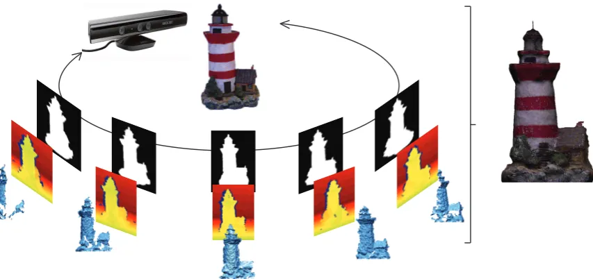
1.1 An example of a 3D reconstruction. The Microsoft Kinect camera is rotated around an object (Lighthouse). Multiple images are captured and silhouette and depth information is extracted. All this information is merged together to generate a 3D reconstruction (right). . . 2

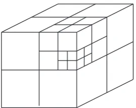
2.1 An example of a silhouette cone intersection on a slice. The object (blue) is seen by two cameras. With more cameras the green areas will be refined, but the concavity (yellow) cannot be recovered with only silhouette information. . . 9 2.2 To improve efficiency an octree representation can be used when doing

a voxel reconstruction. The space is represented as 8 voxels, each voxel can be split into a further 8 voxels until a minimum voxel size is reached. 9 2.3 Given a Lambertian reflection model the colour of the surface of an

object should be consistent from multiple views. This can be used to re-cover concavities, which can be difficult using only silhouette information. 11 2.4 The right image gives an example of the raw data from a time-of-flight

depth camera of the object on the left as presented in [20] . . . 13 2.5 The corners (red) of a standard checkerboard pattern can be used to

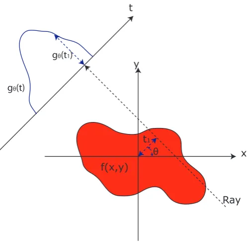
calibrate a standard camera. . . 16 2.6 An example of a Radon transform at an angle θ of a distribution; the

(12)

2.7 The left image is the original image. The middle image shows the Radon transform of that image with each column of the image corresponding to a different angle. The right image shows the reconstruction using the inverse Radon transform. This image is produced using MATLAB’s radon and iradon commands with 180 views. . . 26

3.1 Four images of the Stanford Bunny Object. . . 33 3.2 Four silhouette images of the Stanford Bunny Object, the foreground

pixels are white and the background pixels are black. . . 34 3.3 Image plane and pixel ray (black) with cone like distribution (red), the

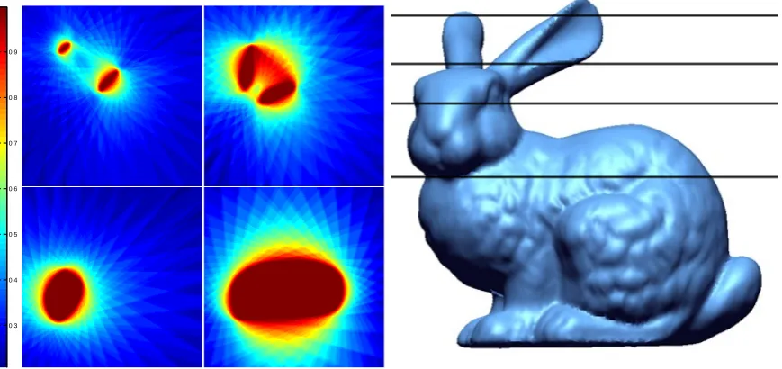
point (blue) can be projected back to the image plane using the cameras projection matrix. . . 36 3.4 The left image shows example slices of regularly sampled likelihood of

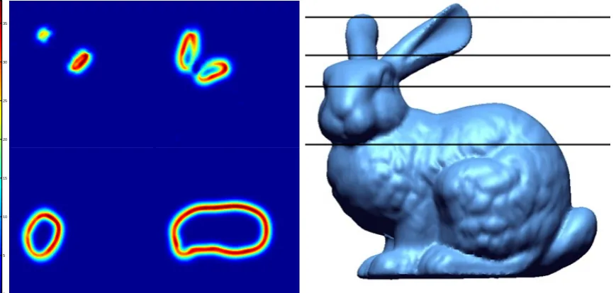
the Stanford Bunny object using 36 cameras andh= 1. The right image shows what slices of the object are being visualised. Top left: Top of the ears, Top right: Middle of the ears, Bottom left: Head, Bottom right: Middle of the body. . . 38 3.5 Example slices of regularly sampled likelihood of the Stanford Bunny

object using different numbers of cameras and h = 1. Top left: 36 cameras, Top right: 12 cameras, Bottom left: 9 cameras, Bottom right: 3 cameras. . . 39 3.6 Two different visualisations of four example slices of regularly sampled

likelihood of the Stanford Bunny object using different bandwidths, number of cameras = 36. Top left: h= 1, Top right h= 2, Bottom left

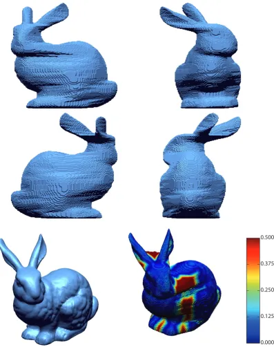
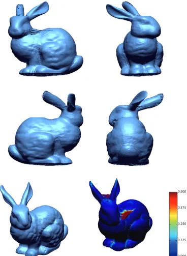
h= 4, Bottom right: h= 8. . . 40 3.7 The top four images are views of the Reconstruction of the Stanford

(13)

3.8 Starting at the bottom of the black line, a point is converged towards higher likelihood along the black line until it reaches the plateau where it stops at the plateau. . . 43 3.9 Starting with a random selection of points (a), the points are converged

to maxima, their path is shown in (b) and finish at the final point loca-tions as shown in (c). . . 45 3.10 Starting with a ring of points (a), the points are converged to maxima,

their path is shown in (b) and finish at the final point locations as shown in (c). . . 46 3.11 Firstly the slice is sparsely sampled. The boundary of this is then turned

into points (a), the points are converged to maxima, their path is shown in (b) and finish at the final point locations as shown in (c). . . 47 3.12 The top four images are views of the Reconstruction of the Stanford

Bunny object using silhouette information and Newton’s Method. The bottom left is the ground truth, the bottom right is an error plot. The scale is 0-0.5 cm on an object of 10 × 13 × 13 cm. The average error is 1.37 mm. When compared with the regular sampling method, it is possible to see the result is much smoother. . . 49 3.13 Four depth images of the Stanford Bunny Object, the darker the pixel

the further away the pixel is from the camera. . . 51 3.14 The combination of the cone from the pixel and the depth information

is combined to give the likelihood of where the corresponding surface point of the object is in the space. . . 53 3.15 Comparison of the two depth models, original model (left) with a pixel

(14)

3.16 An alternative visualisation of the comparison of the two depth models. Here just two data points are in the source data, and this image shows the likelihood model for their locations in the space. The original model (left) with a pixel bandwidth of 1 and a depth bandwidth of 0.0002. The second model (right) just has a depth bandwidth of 0.0002. The different bandwidths allow for a more precise model of the data to be projected, which can change depending on the pixel position. . . 55 3.17 The left image shows example slices of regularly sampled likelihood with

depth information of the Stanford Bunny object using 36 cameras and

h = 1. The right image shows what slices of the object are being visu-alised. Top left: Top of the ears, Top right: Middle of the ears, Bottom left: Head, Bottom right: Middle of the body. . . 56 3.18 Similarly to the silhouette version, 50 random points are selected for

starting positions (left image), they converge to the nearest maxima using Newton’s algorithm. The final locations can be seen in the right image, the problem is the majority of the 50 points have converged to just 4 points on the ridge, not equally spaced as is required for good reconstruction. . . 57 3.19 The likelihood of the surface of an object can be seen as an irregular

ridge (left most image). Due to the irregular height of the ridge, points when converged go to a maxima on the ridge and are not evenly spread along the ridge. By combining a doughnut shaded likelihood (middle image) with the ridge likelihood it is possible to determine a next and previous point along the ridge (right image). The current point ˆΘ(n)_can be seen in black. The possible next points Θ(n+1) _{can be seen in blue on} the top of the peaks in the right image. . . 59 3.20 Four views of the Reconstruction of the Stanford Bunny object using

(15)

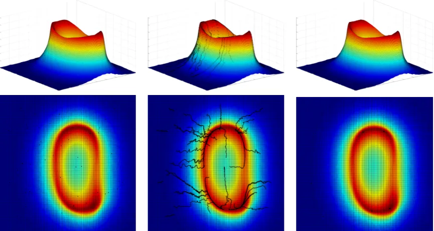
4.1 In the top pair of images the raw data (left) and equivalent likelihood (right) can be seen for a single camera. The middle pair of images shows the addition of a second camera which is not quite aligned properly to the initial data. The bottom pair of images shows the two cameras aligned after finding the best Ψ for the second camera using the Equation 4.18. In this case the points are sampled from the likelihood of the top right image and used to align the second camera. It can be seen that the result in the bottom image has a much better alignment in the raw data and a stronger likelihood in the bottom right image. . . 67 4.2 Example camera alignment. The red cameras show the original position

and orientation of the cameras. The blue cameras show the position and orientation after performing the camera alignment process. . . 72

5.1 A screen shot of the software program Autodesk 3DS Max which was used to generate the synthetic data. . . 75 5.2 The five synthetic objects. . . 77 5.3 A photograph showing an example setup using the Kinect Camera and

rotating platform used to generate the real object data-set. . . 78 5.4 The six real objects acquired using the Kinect Camera. . . 79 5.5 Graph showing the relationship between the raw depth data and the real

world depth units. All the experiments carried out in this work have the object placed between 0.6 and 0.8 meters away from the camera. For this section of the four degree polynomial curve there is a near linear conversion. The consistent standard deviation along this section allows the depth bandwidth to be calculated. This works out at 0.0002m. . . 81 5.6 The two Middlebury objects, the Dino on the left and the Temple on

the right. . . 82 5.7 Example reconstructions of the synthetic objects all using 36 camera

(16)

5.8 Example reconstructions of the real objects all using 36 camera views. The columns from left to right are the original object, the reconstruction from silhouette data using regular sampling, the reconstruction from sil-houette data using Newton’s method and the reconstruction from depth data using Newton’s method and surface explore. . . 86 5.9 Results for Middlebury objects using regular sampling method. These

reconstructions use only silhouette information as no depth information is available for the Middlebury objects. . . 87 5.10 The accuracy of the reconstruction (green) relative to the ground truth

model (blue) is the shortest distance from each point on the reconstruc-tion to the ground truth as shown with the red lines. . . 87 5.11 Going from left to right the resolution of the regular sampling is double

each time, 50, 100 and 200 . . . 89 5.12 Comparison of different regular sampling resolutions and camera

num-bers on the time taken to complete full 3D reconstruction. . . 90 5.13 The left side shows the regular sampled object and the right side shows

the Newton’s method approach . . . 92 5.14 Comparison of different numbers of reconstruction points and camera

numbers on the time taken to complete full 3D reconstruction. . . 93 5.15 The left side shows the object using silhouette information only and the

right side includes depth information . . . 95 5.16 Meshing the raw depth data from the Kinect camera illustrates the

(17)

5.18 For a single slice of a silhouette reconstruction from 36 camera views of the Bunny object (An example silhouette can be seen in the top left image). Different numbers of silhouettes are replaced by silhouettes from another object (the Head object an example silhouette of this object can be seen in the top right image). This is to assess how the model handles contaminated data. Up to nine silhouettes present very little change, however, over that number and it can be seen that the slices are starting to change shape. . . 99 5.19 Example of false limbs being produced. Here only 3 cameras are used to

reconstruct the teapot object using silhouette information alone. Due to overlapping shadows false spouts appear around the object. . . 100 5.20 Example reconstructions with added colour information . . . 101 5.21 Comparison between reconstruction method and laser scan. The top

left image shows an image of the object, the top middle image shows the raw data from the Kinect camera, the top right image shows the reconstruction of the object. The bottom left image shows the raw data from the laser scan of the object and the bottom right image shows the error between the reconstruction and the laser scan. The error bar scale is 0-0.5 cm and the object is 18 × 16×26 cm. The average error is 1.4 mm. . . 102 5.22 Comparison between reconstruction method and laser scan. The top

left image shows an image of the object, the top middle image shows the raw data from the Kinect camera, the top right image shows the reconstruction of the object. The bottom left image shows the raw data from the laser scan of the object and the bottom right image shows the error between the reconstruction and the laser scan. The error bar scale is 0-0.5 cm and the object is 18 × 10 × 27 cm. The average error is 0.765 mm. . . 104

(18)

A.3 Example Kinect Capture. Left is the RGB image, the middle is the projected pattern as seen by the CMOS sensor and the right image is a grayscale representation of the depth with white being far away and the

dark being close to the camera. . . 113

A.4 The glass chessboard used to calibrate the Kinect Camera, both the colour and the depth sensor can see the pattern. . . 115

B.1 Balloon Lady . . . 117

B.2 Clock . . . 118

B.3 Gnome . . . 119

B.4 Lego . . . 120

B.5 Lighthouse . . . 121

B.6 Vanish . . . 122

B.7 Bunny . . . 123

B.8 Dragon . . . 124

B.9 Head . . . 125

B.10 Human . . . 126

B.11 Teapot . . . 127

B.12 Dino . . . 128

B.13 Temple . . . 129

C.1 The pinhole camera model . . . 131

C.2 The corners (red) of a standard checkerboard pattern can be used to calibrate a standard camera. . . 132

E.1 In camera 1, a pixel ut 1 and a camera centre c1 are used to calculate a 3D ray of all possible pointsxt 1,u in the 3D world that project onto pixel ut 1. . . 139

E.2 Two pixels ut_i and ut_j used to calculate point xt by intersection the 2 rays Rt_i,_u and Rt_j,_u. Where camera i= 1 and camera j = 2. . . 140

E.3 Two optical flows used to calculate the scene flow of a point using two sets of intersection rays. Where camera i= 1 and camera j = 2. . . 141

(19)

E.5 Two consecutive frames of the Human Eva II dataset consisting of 4 cameras also the result of the background subtraction and the thresh-olding of the optical flow. . . 145 E.6 Results of the 4 scene flow algorithms. (a) using the background

subtrac-tion, (b) thresholding the optical flow, (c) thresholding the scene flow and (d) exploring the histogram data. The computation time for each scenario is (a) 1.8 seconds (b) 1.4 seconds (c) 7.9 seconds and (d) 117 seconds. This does not include the time taken to calculate the optical flow or background subtraction. . . 147 E.7 The scene flow result obtained using the background subtraction is

pro-jected back into camera 4, and the magnitude of the difference between the original optical flow and the new optical flow is plotted. . . 147

F.1 Room layout with cameras, motion capture cameras and calibration tools.149 F.2 An example capture showing the six images taken simultaneously and

(20)

Chapter 1 Introduction

3D reconstruction is one of the most basic and important tasks in a multi-camera system. It is the process of combining multiple 2D images together to form a 3D model of the object of interest. It serves as a foundation for numerous higher-level applications in many domains including motion capture, 3D recognition and 3D modelling. An example of a 3D reconstruction can be seen in Figure 1.1. In this thesis a novel framework for merging data from a multi-camera system to produce a flexible system for 3D reconstruction is proposed. Examples are given for how the framework performs using both synthetic data and real world data and show how the same framework can be used to help optimise camera alignment.

1.1 3D Reconstruction Challenges

3D reconstruction can be a very challenging problem. The reason for this can be broadly broken down into three main factors: converting from 2D information to 3D information, the nature of the object, and the considerable noise in the acquisition system.

• The information available is generally 2D images. To perform a 3D reconstruction it is necessary to calculate the 3rd dimension with no other information. This is not a trivial task. Depth cameras can be used to help in this respect.

(21)

[image:21.595.110.537.133.334.2]

Figure 1.1: An example of a 3D reconstruction. The Microsoft Kinect camera is rotated around an object (Lighthouse). Multiple images are captured and silhouette and depth information is extracted. All this information is merged together to generate a 3D reconstruction (right).

infer the shape of the object. Here no such prior knowledge is available, only the information from the images is available.

• Noise increases the difficulty of this problem considerably. Noise altering the quality of the images and uncertainty in the camera parameters can cause errors in the reconstruction. Noise in the appearance of the object due to light variations and other noises can all cause problems when attempting to reconstruct an object.

1.2 Motivations

(22)

sav-hours of work by expensive skilled workers.

• Object Recognition - Identifying and recognising objects in ordinary images is a highly active area of research in computer vision. While this is normally done using 2D images there has been a move towards using 3D reconstructions as they can help with the recognition process even with variations in pose and illumination that can be problematic when only using 2D images. This requires firstly generating the 3D reconstruction before it can be recognised.

• Stereo - Recent years have shown an increase in 3D movies. These movies use stereo camera rigs, or multi-camera rigs to capture the movie to create the 3D effect. It is possible to use these multi-camera setups to also do partial or full 3D reconstructions of the scene. This is useful for postprocessing where artifacts have to be removed, like stunt man wires, or corrected, or to add special effects into the scene.

• First step towards other problems - Many higher level computer vision tasks use 3D reconstruction as a first step towards their goal, for example Markerless Motion Capture which is the tracking and capturing of the movement of a human and their limbs. One method to achieve this is to do repeated 3D reconstructions at regular time intervals. Another area is Human Computer Interface where a person can pose or gesture and it will be recognised by the computer to perform an action. 3D reconstruction can be used to help determine the persons pose or gesture.

1.3 Goal

The goal of this thesis is to develop a new multi-view 3D reconstruction framework with the following characteristics:

(23)

• A statistical approach capable of modelling directly the noise of all the input data from the sensors at a fundamental level, without the need for multiple stages to remove outliers or to smooth data.

• Be suitable to take advantage of the latest parallel computer architectures to allow for fast reconstructions.

1.4 Contributions and Thesis Outline

The main contribution of this thesis is a new statistical framework for 3D reconstruction which is based on the generalised Radon transform. An explanation of the generalised Radon transform and an overview of the current state of the art on 3D reconstruction methods is presented in Chapter 2. The framework is designed to do a 3D reconstruc-tion and infer the shape of an object of interest from multi-view data and is presented at the beginning of Chapter 3. The generalised Radon transform is extended to be-come the generalised relaxed Radon transform which can be linked to kernel density estimates (also explained in Chapter 2).

(24)

but also capturing the depth at each pixel in the image from the camera to the corre-sponding point in the scene. This represents a considerable increase in information that can be used in the reconstruction but depth information captured by current hardware can be exceptionally noisy and this noise must be considered when generating a 3D reconstruction from depth information.

The framework is extended in Chapter 4 to find the optimal value of the camera parameters. Techniques exist which allow for a good initial estimation of the camera parameters to be calculated. Camera parameters are the position and orientation of the camera in space and the internal variables which allow a point in space to be pro-jected into the image plane. While the internal variables can be accurately calculated the position and orientation can be prone to error. Accurate camera parameters are es-sential for recovering fine detail in the reconstruction. This extension of the framework allows for these uncertainties to be taken into account and helps improve the aligning of the cameras together.

Chapter 5 applies the reconstruction techniques to a variety of objects and compares and contrasts the different methods and effects of different parameters. Two data-sets were created to test and evaluate these reconstruction methods. The first data-set is a synthetic data-set created using software. This allows full control of all the parameters and settings. The synthetic data-set was created from 3D models. These models can therefore be used as ground truths to allow full quantitative evaluations to be performed. The second data-set was created using the new Microsoft Kinect camera, which is capable of also capturing depth data. Data for numerous objects was captured, the objects reconstructed and a full evaluation was performed.

Chapter 6 summarises all the work done in this thesis and concludes this research by outlining possible future directions of investigation.

1.5 Publications to Date

During the course of this thesis the following publications were produced:

(25)

E.

• Jonathan Ruttle, Michael Manzke, Martin Prazak and Rozenn Dahyot. Syn-chronized real-time multi-sensor motion capture system. In SIGGRAPH Asia sketch Poster, page 50:1-50:1, 2009 [87]. This work is presented in Appendix F.

• Donghoon Kim, Jonathan Ruttle and Rozenn Dahyot. 3D shape estimation from silhouettes using mean-shift, in IEEE International Conference on Acoustics, Speech and Signal Processing, pages 1430-1433, 2010 [51]. This work is summarised in the state of the art Section 2.3.3.

• Jonathan Ruttle, Michael Manzke and Rozenn Dahyot. Smooth kernel density estimate for multiple view reconstruction, in Conference on Visual Media Production, pages 74-81, 2010 [86]. This work is presented in Section 3.2.

(26)

Chapter 2 State of the Art

In this chapter, the past works on 3D multi-view reconstruction (Section 2.1), camera calibration (Section 2.2), inference with kernel modelling (Section 2.3) and the gen-eralised Radon transform (GRT) (Section 2.4) are reviewed. Visual hull, a common approach for 3D shape inference, is an essential step in 3D reconstruction that is of-ten modelled using a discrete objective function. This objective function corresponds to a 3D histogram and can be changed to a smooth differentiable objective function using kernel modelling. It is proposed that 3D volumes are inferred by using the gra-dient ascent method optimising a kernel mixture (Section 2.3.2). Finally the GRT is introduced as it is at the core of the work presented later in this thesis.

2.1 3D Multi-View Reconstruction

Seitzet al. [90] provides a good summary of the field where they split the reconstruction up into four categories. The first category of techniques computes a discontinuous cost function on a 3D volume as a 3D histogram [91, 13, 7]. The second category involves iteratively evolving a surface to decrease or minimise a cost function [28, 55, 4]. The third category uses depth information computed on each pair of images which it then merges together to produce the end result [14]. The fourth category of algorithms does matching across images from which surface points can be estimated [78].

(27)

volume to produce an initial estimate of the shape and size of the object as in the first category. This would give an estimate of the surface which can be improved using algorithms from the second category which are based on either depth estimation or surface point matching from the third and fourth categories. This results in a pipeline of processes, each with the goal of providing further raw data for a further stage of the pipeline or refining the current mesh to produce higher accuracy [109, 88].

Another way to categorise the different algorithms at a more basic level is in the different information used behind the method. The next set of subsections describe some 3D reconstruction algorithms; firstly from silhouette information, secondly from colour information and thirdly from depth information.

2.1.1 Shape from Silhouette

The visual hull is a geometric entity created by shape-from-silhouette 3D reconstruction techniques introduced by Martin et al. [67]. This method assumes the foreground object in an image can be separated from the background. This foreground object, also known as a silhouette, is the 2D projection of the corresponding 3D foreground object. Along with the camera viewing parameters, the silhouette defines a back-projected generalised cone that contains the object. The intersection of two or more such cones is called the visual hull (Figure 2.1).

In practice this method is accomplished by dividing the world up into regular 3D volumes called voxels (volume elements). In turn each voxel is projected onto each image plane and if the corresponding pixels in each of the image planes are foreground pixels then the voxel is assumed to be part of the visual hull. If the projected pixels are background pixels then the voxel is assumed to be transparent.

(28)

[image:28.595.253.388.526.633.2]

Figure 2.1: An example of a silhouette cone intersection on a slice. The object (blue) is seen by two cameras. With more cameras the green areas will be refined, but the concavity (yellow) cannot be recovered with only silhouette information.

(29)

This type of shape-from-silhouette method can produce a reconstruction that is guaranteed to enclose the true object but is unable to recover surface concavities in the object [56]. The quality of the resulting 3D reconstruction greatly depends on the number of viewpoints and the accuracy of segmenting the image into foreground and background pixels. The 3D reconstruction can suffer from self occlusions but this prob-lem can be partially resolved with greater number of viewpoints. The minimum size of the voxel also greatly affects the end quality of the reconstruction; the smaller the voxel the greater the quality. Unfortunately the computation time and memory requirement are directly linked with the size of the voxel and as the voxel is made smaller, the time and memory requirement increase. Many 3D reconstruction algorithms are variations on this method, all designed to generate a visual hull [27, 11, 57, 97, 69, 99, 32]. Once the solid voxel representation is generated it is generally required to convert it into a 3D mesh. This can be done using a method called Marching Cubes which will discover the edge voxels so that they can be converted into mesh vertices [62].

2.1.2 Shape from Photo-Consistency

Seitzet al. [91] proposed an extension to the visual hull called the photo hull. The idea behind the photo hull is to use colour consistency instead of just geometric intersection of silhouette cones. If a voxel has consistent colour across all the image planes that can see it, then it is deemed to be part of the surface of the object. If the colours are inconsistent, then the voxel is deemed to be transparent. This method of repeated classification of voxels is called space carving and is used until all the voxels are deemed colour consistent, transparent, or not visible (inside the object). The end result of the method is a set of coloured voxels which is called the photo hull.

(30)

(a) (b)

Figure 2.3: Given a Lambertian reflection model the colour of the surface of an object should be consistent from multiple views. This can be used to recover concavities, which can be difficult using only silhouette information.

a Lambertian reflection model, meaning light falling on it is scattered such that the apparent brightness of the surface to an observer is the same regardless of the observer’s angle of view. Therefore, the colour of the surface point should look the same from any viewpoint that can see it. A number of variations of this method have been proposed that use different methods of determining colour consistency and employ optimisations in the data structure to suit the algorithm [55, 96, 95, 1, 53].

2.1.3 Shape from Stereo Pairs

Stereopsis is another highly active field of computer vision research. The idea behind stereopsis is similar to that of the human vision system. Two nearby views of the same scene are taken at the same time. By matching points in one image to the other image it is possible using the two cameras’ geometry to calculate the 3D position of that point in space. Repeating this for as many points as possible in the scene gives a point cloud that can represent the scene. This can be used to generate a 3D reconstruction of one side of the object. By using multiple sets of stereo pairs of cameras it is possible to produce a point cloud from each stereo pair and merge them together to produce a full reconstruction.

Scharstein and Szeliski [89] produced a comprehensive review of dense two-frame stereo algorithms in 2002. The following is a very short outline of stereo algorithms which have been used to do full 3D reconstructions. For further information [89] is a good place to start.

(31)

from the left image is matched to the same point, patch or feature in the right image. Corner and edge detection as proposed by Harris and Stephens was one of the first feature based matching methods; edges and corners in one image should correspond to corners and edges in another image [42]. More advanced feature methods then were developed such as the Scale-Invariant Feature Transform (SIFT) method [63] which provides a way to detect and describe features in a scale-invariant manner to make it easier to match. The distance between the camera centres (baseline) is an important factor in stereo vision; the further away the cameras are, the harder it is for good robust feature matches to be made. Mataset al. proposed Maximally Stable Extremal Regions (MSER) [68] are suitable for this type of feature matching. In order to speed up stereo matching Bayet al. proposed Speeded Up Robust Feature (SURF) [2] which is based on 2D Haar wavelets and which are very fast to calculate. Other features exist as seen in [70, 104]. Mikolajezyk and Schmid gave a good review of common local descriptors [71]. To improve the task of matching it is possible to rectify the images. This is where the images are aligned in such a way that each line in one image corresponds to a line in the other image [35]. This means that a 2D search of the whole image for a match can be reduced to a 1D search of the corresponding line in the other image.

Once the matches are made and the camera geometry is used to calculate real world position of the points, it is then required to merge the points together. A number of methods have been proposed to accomplish this. It is important to be robust to outliers. When points are matched incorrectly those points will be useless for the reconstruction and must be removed before continuing [14, 58]. A number of methods use an initial step of generating a visual hull from silhouette images. This assists with merging the stereo information and removing outliers [29, 16, 48].

(32)

Figure 2.4: The right image gives an example of the raw data from a time-of-flight depth camera of the object on the left as presented in [20]

2.1.4 Shape from Depth

If a depth sensor is available, then the stereo matching stage from the previous section can be skipped and the problem becomes focused on merging together the point clouds to create the 3D reconstruction. The problem that arises in this situation is that the depth data from the sensors is generally very noisy, as seen in Figure 2.4, and must be smoothed to some extent before being used. Another problem that can arise is aligning the depth data together to the same world space so that all the depth data aligns correctly. Both Cuiet al. [20] and Reynolds et al. [82] have proposed methods which help solve these problems both on an object scale and in a scene scale.

With the introduction of the Microsoft Kinect sensor in November 2010 there has been a large increase in the number of methods introduced for 3D reconstruction from depth information. This is because the Kinect sensor is the first low cost (∼e150), mass produced and relatively high resolution (640×480 pixels)depth sensor to be intro-duced into the market. Previous to the Kinect sensor, depth cameras were extremely expensive (>e1000) and had relatively low resolution (< 320 × 240 pixels). More information on the Kinect sensor can be found in Appendix A.

(33)

Kinect sensor that has been proposed in papers by Izadi et al. [47] and Newcombe

et al. [72]. The KinectFusion method continuously tracks the six degrees of freedom pose of the camera and fuses new viewpoints of the scene into a global surface-based representation. An iterative closest point algorithm is used to calculate the relative six degrees-of-freedom transformation from the current view-point to that of the previous frame to perform the continuous tracking. The newly aligned data is then added to the growing reconstruction which is a voxel based volumetric representation. The method uses a GPU implementation to be able to give real-time results. The method relies on small movement between frames to calculate a good transformation from the current view-point to that of the next and has considerable memory requirements in terms of it’s voxel based volumetric representation.

2.1.5 Shape from Other Information

There are a number of other methods which can be used to generate 3D reconstruc-tions. For example, some methods use the normals of the silhouette edges in the image plane. The normal of the silhouette edges are the 2D projections of the 3D normal of the surface of the object and they can be used to generate a 3D reconstruction [60]. Different methods of using multi-resolution representation of the raw data are proposed by Manson et al. [66] which uses wavelets to help reconstruct a surface mesh. Paris

et al. propose a method based on graph cuts which is used to minimise the distance between the estimate of the reconstruction and the data from the images [74].

2.1.6 Remarks

(34)

from different sources together, to produce a more accurate and complete reconstruc-tion than any one stage or method could on their own. The disadvantage of this type of pipeline is that in each stage decisions have to be made in terms of matching points or threshold levels, and with each decision errors can be made. Information can be lost and bad information can be propagated through to the next stage. Extra stages can be added to the pipeline to remove any outlier or error to reduce their further effect, but very little can be done to recover any information that may be lost.

These two areas are considered in this thesis as the two major bottlenecks or prob-lem areas for the future of 3D reconstruction methods. The goal, therefore, of this thesis is to develop a framework which tackles the 3D reconstruction problem from a different direction. Instead of an objective function that is discrete, here a smooth continuous and differentiable function is defined that can be optimised using a gradient ascent algorithm. This framework has the flexibility to allow all the same information to be used, but combined all together at the same time, with the accuracy of each sen-sor modelled at a fundamental level and includes tools and techniques that will make the problem of scaling in dimensionality and resolution a feasible and affordable cost. The future of computer processing architecture is highly focused on multi-core solu-tions and many of the latest techniques are focusing on massively parallel architectures like multi-core CPUs and GPUs. Therefore, it is also important that the framework should be suitable and designed to take advantage of such architectures.

2.2 Camera Calibration

The procedure for determining the intrinsic and extrinsic camera parameters is called camera calibration. Intrinsic parameters are particular to the internals of a specific camera including the focal length, center point and radial distortion coefficients. These intrinsic parameters may change as a camera’s focus and magnification is changed. The extrinsic parameters place the camera at a particular point in the world relative to a known origin. Many methods are available for determining the camera parameters [43]. The choice of the method generally depends on the prior information available and the situation for which the camera calibration is required.

(35)

X Y

O 50

100

150

200

250

300

350

400

450

Figure 2.5: The corners (red) of a standard checkerboard pattern can be used to calibrate a standard camera.

the corners of the checkerboard in the real world and the corresponding coordinates of the projection of those corners in the image plane can be used to solve for the camera parameters. Since the projection matrix contains 12 entries and 11 degrees of freedom, a minimum of five and a half 3D to 2D projections are needed, since each projection contains two relationshipsxandy. To overcome problems due to noise, normally many more points are used and an optimisation process is used to solve for the unknown parameters both extrinsic and intrinsic. Coefficients for radial distortion can also be calculated using this method. For a standard camera left in the one configuration it is possible to only calculate the intrinsic parameters once and then only one image of a checkerboard is needed to calculate the extrinsic parameters for each viewpoint required.

For a multi-camera system, common points should be used to guarantee that all the cameras have a common world origin and are correctly positioned relative to each other. A MATLAB toolbox has been developed by Bouguet and has been used for all the camera calibration in this work [9].

(36)

work backwards (with the assumption that the scene stays static) and calculate the movement of the camera relative to the objects. This method requires large overlap between viewpoints of the scene, so good optical flow can be calculated. It works best with a slowly moving camera with a high frame rate resulting in very little movement which can be accurately tracked over time. The accuracy of this method depends on the accuracy of the optical flow calculations. To improve this, the optical flow and camera movement can be calculated over numerous frames and the result smoothed and interpolated to correct for any noise.

2.3 Inference using Kernel Density Estimates

2.3.1 Kernel Density Estimation

Kernel density estimation is a method for estimating a probability density function. The method was first proposed by Rosenblatt [84] and later expanded by Parzen [75], who added multiple different kernel types. The basis of kernel density estimation is that given a sequence of independent identically distributed random variablesx1, x2, . . . , xn, with a common probability density functionf(x) then the kernel density estimate ˆf(x) will be:

ˆ

f(x) = 1

nh n X i=0 k

x−xi

h

(2.1)

where k is the kernel, and h > 0 is a smoothing parameter called the bandwidth. A number of different kernels can be used. The requirements for a kernel are that it should be symmetric and that it should integrate to one. The most common kernel used is the Gaussian kernel as seen in Equation 2.2, and while there are many alternative kernels, the Gaussian kernel is the one that is used throughout this thesis.

k(x) = √1

2π exp

−x 2 2 (2.2)

(37)

have the bandwidth as small as possible to preserve as much detail and structure as possible but large enough to overcome any noise in the input.

2.3.2 Stochastic Exploration

There is a great deal of literature covering the area of stochastic exploration, but two books in particular give an excellent detailed explanation of the subject; chapter 5 of Monte Carlo Statistical Methods [83], and chapter 9 of Convex Optimization [10]. The following section gives an overview of stochastic exploration as it is applied in this thesis. For more information, please refer to these two books.

In general the goal is to solve and optimise the problem of:

arg max x

f(x) (2.3)

It is assumed that f is convex and twice differentiable. It is also assumed that there exists an optimal pointx∗; a solution to the problem in Equation 2.3. In certain situations the problem can be solved analytically by solving the set of equations:

∇f(x∗) = 0 (2.4)

where ∇f is the gradient of the function. In all cases the maxima or minima of the functionf should have a gradient equal to zero. Therefore, solving for x when the gradient equals zero should solve the problem.

Realistically, in most cases of interest, the problem is too complex to be solved analytically. An alternative to solving the problem in Equation 2.3 is called regular sampling. Regular sampling is a method where the domain of the function is broken up into small regular intervals and the value calculated per interval. The result can be thresholded to give a solution to the problem. In practice, regular sampling can be computationally very expensive and the accuracy of the result depends highly on the resolution of the regular sampling. Therefore, to increase the accuracy has a considerable effect on the computational cost.

(38)

sequence. Many iterative algorithms exist. One such algorithm is the mean-shift algorithm. While not a major focus in this work, an overview of its use is given in the section below. Another area of algorithms is the gradient ascent algorithms which includes Newton’s method. Newton’s method is widely used in the work in this thesis and is fully explained in the sections below.

Mean-Shift

A mean-shift method is a non-parametric mode-seeking algorithm, which climbs the gradient of a probability distribution to find the nearest domain mode (peak). The algo-rithm was originally proposed by Fukunaga and Hostetler [33]. Cheng [15] generalised the method and introduced it to the image analysis field with a mode-seeking process on the density function surface. More recently, Comaniciu and Meer [18] proposed practical applications such as segmentation, tracking [19, 17], etc. The convergence of the mean-shift is proven for the Gaussian kernel in [15] and for any kernels with a convex and monotonically decreasing profile, such as the Epanechnikov kernel in [18]. It has been shown that mean-shift can be used on high dimension problems such as texture classification [36].

Gradient Ascent

The general ascent algorithm is as follows:

Algorithm 1: General Ascent Algorithm

given a starting point x(0)

repeat

1. Determine ascent direction ∆x

2. Choose a step sizet >0 3. Update x(n+1) ₌_x(n)₊_t_∆_x

until stopping criterion is satisfied

(39)

Ascent Direction The first ascent direction that can be used is the gradient∇f(x) of the function f at the point x. This method exhibits approximately linear con-vergence. Many different ascent directions can be used such as steepest ascent. In practice the Newton Step has been shown to converge faster than most methods with a quadratic convergence rate. The Newton direction is:

∆xnt = [Hf(x)]−1∇f(x) (2.5) where Hf(x) is the Hessian matrix of the functionf.

While the gradient will always give a direction that increases, the Newton direction gives the direction that may point in either the increasing or decreasing direction. This depends on whether it is closer to a maxima or a minima and on the underlying function being maximised. It is possible to do a dot product between the gradient and the Newton step to determine if it is heading in the correct direction. A positive result is correct; a negative result means the direction needs to be inverted. This can be done by multiplying the direction by minus one. One alternative to this is to compare the value of the function before and after the jump. If the value of the function has decreased then the direction of the jump can be reversed.

(40)

One such line searching algorithm used is called backtracking. Backtracking uses two constantsα and β where 0< α <0.5 and 0< β <1.

Algorithm 2: Backtracking line search

given a descent direction ∆x and α ∈(0,0.5) andβ ∈(0,1)

t= 1

while f(x+t∆x)< f(x) +αt∇f(x)T_∆_x _do

t=βt

end

Stopping Criterion A very important part of using Newton’s method is the stop-ping criteria. A number of methods can be used to determine when to stop jumstop-ping towards the maxima. The most common is to define a threshold and when the jump distance is smaller than this threshold, stop jumping. A similar method of thresholding can be applied to the change in value of the function between one point and the next. If the value decreases this can be a sign that it has gone beyond the maxima, but this might also be due to the problem mentioned above where Newton’s method will just as easily converge towards a minima. Another method also used is to define a maximum number of jumps. This can be used bearing in mind that if the point has not converged towards the maxima within that number of jumps it may be deemed to be following some random noise in a random direction. Therefore, it is better to stop after that maximum number of jumps and start again somewhere else.

(41)

Simulated Annealing

Simulated Annealing is a method where the the scale of the problem is changed to allow for faster convergence. It also helps avoid the trapping attraction of local maxima and focus on global maxima. In this case the scale of the problem can be changed by increasing the bandwidth of the underlying kernel. Increasing the bandwidth can incur some other problems, as it can remove the fine detail of an object. Therefore, as the point converges towards the global maxima the bandwidth can be decreased; similar to the method used by Shenet al. [92]. It is possible to use a simulated annealing scheme which will start with a large bandwidth hmax and decrease it iteratively towards a minimum bandwidthhmin as the point converges to a global maxima. This is generally done at a geometric rate.

ht=αthmax until ht=hmin with 0< α <1 (2.6) It has been shown that the speed of meshift can be improved by using an an-nealing method [52, 22].

Overall Newton’s Method of optimisation has been shown to be more efficient (re-quires fewer steps to converge) than mean-shift and makes fewer assumptions on the form of the underlying kernel structure [39]. In general mean-shift requires a linear kernel structure but a Newton-style only requires the kernel to be differentiable to the second order to fit the equation.

A number of papers have used these types of gradient ascent algorithm to solve a number of problems in computer vision. The most popular of which are tracking algorithms [26, 30, 31, 92].

Parallel Computing

The mean-shift algorithm has been shown to be easily parallelled and can be pro-grammed for a GPU as shown by Li and Xiao [59].

(42)

compu-2.3.3

Inference of Visual Hull using Kernel Modelling

As noted in Section 2.1.6 most 3D reconstruction methods focus on discrete objective functions. By using kernel modelling it is possible to generate smooth objective func-tions. Work that has been done towards this goal was to define a continuous objective function for an orthographic camera model 1.

ˆ

p(x)∝ 1

n N X i=1 1 √

2πhexp

−(ρi−xcosθi−ysinθi)2 2h2

!

(2.7)

In this work x = (x, y) the latent point of interest on a 2D slice and {ρiθi}i=1,...,N are a set of N independent observations which represent the rays corresponding to silhouette pixels from all the orthographic cameras.

This results in a continuous representation of the space which can not only be explored using regular sampling techniques but can also be explored using mean-shift gradient ascent techniques to reconstruct the object of interest. This work allowed all information to be considered in a continuous likelihood, where all information is weighted and combined together.

Limitations exist in respect of the orthographic camera model used as the basis of the algorithm which is mainly used for medical images as compared to the pin-hole camera model which is more widely used. Also the mean-shift algorithm used is not suitable to work with the more complex pin-hole camera model as it requires a linear mathematical model or a linear approximation to work. Kim’s work [50] shows that the framework can be extended to include colour and prior information which improves the accuracy and completeness of the reconstruction.

2.4 Generalised Radon Transform

The framework which is presented in the next chapter has at its core the generalised Radon transform. Therefore, this section describes the classic Radon transform and the generalised Radon transform and some of the applications to which they have been applied.

(43)

2.4.1 Radon Transform

In 1917 Johann Radon proposed the Radon transform [80] for a function f(x) as:

R[f(x)](p, ξ) = Z

f(x)δ(p−ξx)dx (2.8) where:

• f(x)∈ S(_Rm_{) is a function that is infinitely differentiable}

• dx=dx1, . . . , dxm is a volume element

• ξ = (ξ1, . . . , ξm) is a unit vector that defines the orientation of a hyperplane with equation p=ξx

• δ() is the Dirac delta function

This equation provides the mathematical framework for a great number of recon-struction problems in physics, geology, medical imaging and other areas. A 2D example of the Radon transform can be seen in Figures 2.6 and 2.7. The Radon transform is widely applicable to tomography and tomographic reconstruction, for example, com-puted axial tomography (CAT scan) and magnetic resonance imaging (MRI). An ex-plicit and computationally efficient inversion algorithm exists for 2D Radon transforms called filtered back-projection. Many algorithms have been developed which use the Radon transform [65, 81, 49, 24].

The Hough transform is conceptually very close to the two-dimensional Radon transform; they can be seen as different ways of looking at the same transform [23]. The Hough transform can be seen as a discrete form of the Radon transform and it is mainly used for detecting lines in a 2D image [24, 21].

(44)

x y

t

f(x,y) t1

θ

Ray gθ(t)

[image:44.595.203.454.260.505.2]

gθ(t1)

(45)

Figure 2.7: The left image is the original image. The middle image shows the Radon transform of that image with each column of the image corresponding to a different angle. The right image shows the reconstruction using the inverse Radon transform. This image is produced using MATLAB’s radon and iradon commands with 180 views.

Whereas in the x-ray situation, density information is used which enables the inside of the object to be seen, using only the silhouette information, the surface of the object can be reconstructed. Kim et al. [51], mentioned above, compared their method to this approach due to the similar assumption of an orthographic camera model.

2.4.2 Generalised Radon Transform

Over the years the Radon transform has been generalised [25]; it can be defined in many ways. The generalised Radon transform associated with the equationλ+F(x,Θ) = 0 is:

R[f(x)](Θ, λ) = Z

Rdx

A(x,Θ) f(x) δ(λ+F(x,Θ)) dx

with x∈_Rdx_, _Θ_∈

RdΘ, and λ∈R

(2.9)

(46)

at (Θ, λ) [25]. The integral 2.9 can be equivalently rewritten as:

R[f(x)](Θ, λ) = Z

D

A(x,Θ)f(x)dx (2.10) where the domainD ⊂_Rdx _{is defined as:}

D={x∈_Rdx_|_λ₊_F₍_x_,_{Θ) = 0}_}_. _(2.11)

The generalised Radon transform can be used as a technique for detecting parame-terised shapes, for example, curves, circles and even hyper-sphere in larger dimensions. The way this works is, if given a mathematical model of the shape, the generalised Radon transform can be used to derive a mapping from an image or object space onto a parameter space. The axes of the parameter space corresponds to the parameters of the model. Applying the transform to an image, any shape fitting the model will result in peaks in the parameter space corresponding to the parameters of the shapes in the image [44].

Once this mapping is derived then the problem shifts to finding the peaks in the pa-rameter space. The majority of techniques divide up the papa-rameter space into discrete bins then, either choosing a point in the parameter space and computing its value by integrating the image or object space over all the points that belong to it, or choosing a point in the image or object space and adding its contribution to the appropriate bin in the parameter space; a process known as voting. Then either by exploring the entire parameter space or iterating over all the points in the image or object space, it is possible to detect the peaks in the parameter space.

The generalised Radon transform is widely used for pattern detection. Toft used a discrete form of the generalised Radon transform to detect curves in noisy images [103]. Hansen and Toft used a similar discrete generalised Radon transform to identify hyperbolas of particular interest from seismic data [41].

2.5 Conclusion

(47)

(48)

Chapter 3 Generalised Relaxed Radon

Transform for 3D Reconstruction

This chapter presents an overview of the statistical framework used as the foundation of the work being presented. Firstly a generic derivation of the framework is described. Once the generic framework is outlined then the two specific applications of the frame-work which have been developed and tested are presented.

3.1 Generalised Relaxed Radon Transform

The equation associated with the generalised Radon transform in the state of the art wasλ+F(x,Θ) = 0 as seen in Equation 2.9. A random variable ε can be introduced and that equation can be rewritten as:

λ+F(x,Θ) =ε∼δ(ε) (3.1)

F is a known link function that models the relationship between a latent random vector of interest Θ, and a random vector x for which N independent observations

(49)

pε(ε) other than the Dirac function.

λ+F(x,Θ) =ε ∼pε(ε) (3.2)

For now, no explicit meaning is given to any of the variables and they are just considered random variables. The meaning of the variables will be explained later in the context of the applications (see Sections 3.2 and 3.3).

In summary:

• Θ = [θ1, θ2,· · ·] is the latent random vector of interest.

• x = [x1, x2,· · ·] is a random vector for which N independent observations have been collected {x(i) _{= [}_x(i)

1 , x (i)

2 ,· · ·]}i=1,···,N

• λ is an additive variable. For statistical reasons it is useful to have an additive variable in this situation as it helps with the derivation of the framework. For the applications considered in this thesis, the only case of interest will be when

λ = 0. Other application may use this additive variable if it fits in with the modelling.

• ε is an explicit random variable modelling the perturbation or noise. It has a known distribution pε(ε).

• F is a given function that models the relationship between the variablesx, Θ,ε.

F is defined as F :_Rdim(x)_×

Rdim(Θ)→Rdim(ε) (note that dim(ε) = dim(λ)).

Given the observation variablex, the latent variable of interest Θ and the Equation 3.2, the probability density function ofλ can be written as:

pλ|x,Θ(λ|x,Θ) =pε(λ+F(x,Θ)) (3.3)

The joint probability density function of Θ and λ can be computed by first con-sidering the joint probability density function of Θ, x and λ, expanded using Bayes’ Theorem and then integrating with respect to x.

(50)

pΘ,λ(Θ,λ) =

Z

pλ|x,Θ(λ|x,Θ) px,Θ(x,Θ)dx (3.5)

Equation 3.3 can be substituted in for pλ|x,Θ(λ|x,Θ) and again Bayes’ Theorem can be used to expandpx,Θ(x,Θ).

pΘ,λ(Θ,λ) =

Z

pε(λ+F(x,Θ)) pΘ|x(Θ|x)px(x)dx (3.6)

It should be noted that this is very similar to the generalised Radon transform as seen in the state of the art Section 2.4 Equation 2.9, with px(x) equivalent to f(x),

pΘ|x(Θ|x) equivalent to A(x,u), λ equivalent to c and F(x,Θ) equivalent to I(x,u).

The major difference is where originally the distribution ofε was modelled by a Dirac function, now this assumption is relaxed and the perturbation or noise is modelled with a known distributionpε(ε), therefore, giving rise to the generalised relaxed Radon

transform.

Solving the integration gives the expectation with respect to x.

pΘ,λ(Θ,λ) = Ex[ pε(λ+F(x,Θ)) pΘ|x(Θ|x)] (3.7)

For the moment, within the framework the only known knowledge considered is Equation 3.2. Thus, with no other knowledge, we assume that Θ is independent ofx, therefore,pΘ|x(Θ|x) =pΘ(Θ) and can therefore be taken out of the expectation. Thus

pΘ(Θ) is now a prior on the latent variable. If additional information were available linking Θ and x, then this could be included in the framework. For example, in the Statistical Hough Transform proposed by Dahyot, additional information from the gradient of the image is used to provide an additional link between the latent variable of interest and the observation [21].

pΘ,λ(Θ,λ) =pΘ(Θ)×Ex[ pε(λ+F(x,Θ))] (3.8)

The joint probability density function pΘ,λ(Θ,λ) can be approximated using the

(51)

expected joint probability density function ˆpΘ,λ(Θ,λ) can be seen as:

ˆ

pΘ,λ(Θ,λ) =pΘ(Θ) | {z } prior × 1 N N X i=1

pε(λ+F(x(i),Θ))

| {z }

Averaged likelihood

(3.9)

In the caseλ= 0, results in:

ˆ

pΘ,λ(Θ,λ= 0) =pΘ(Θ)×lik(Θ) (3.10) where

lik(Θ) = 1

N

N X

i=1

pε(F(x(i),Θ)) (3.11)

In particular the averaged likelihoodlik(Θ) as defined above is what is used through-out this work for inferring the latent variable Θ.

3.2 Application 1: 3D Reconstruction using

Silhou-ette Information

The averaged likelihood lik(Θ) can be used to infer the 3D shape of an object from multiple silhouette images of that object to create a Visual Hull 1_.

The Stanford Bunny is a computer graphics 3D test model and it will be used as an example object throughout this work. Four images of the object can be seen in Figure 3.1.

The input in this application is a set of silhouette images where the image has been segmented and the foreground pixels are white and the background pixels are black. Four sample silhouette images of the Stanford Bunny can be seen in Figure 3.2.

For each silhouette image there is also a known 4×3 camera projection matrix. In this case our observations are the white foreground pixels across all the images, in totalN foreground pixels. Each pixel has a pixel coordinate (x1, x2) and an associated

1_{This application has been published in 2010 in the Conference on Visual Media Production}

(52)

(53)

[image:53.595.101.541.214.581.2]

(54)

4×3 camera projection matrix:



 

x3 x4 x5 x6

x7 x8 x9 x10

x11 x12 x13 x14 



 (3.12)

The latent variable of interest Θ = (θ1, θ2, θ3) is the 3D coordinate in the real world. Each foreground pixel can be projected out into the world using the projection matrix. This can be seen as a ray starting from the camera centre and travelling through that pixel in the image plane and out into the world. As the ray travels further away from the camera centre it diverges from its neighbour’s pixels. Therefore, it is better to visualise each pixel as a cone. The pointed end of the cone starts at the camera centre and travels through the pixel and out into the real world, getting bigger as it does. In fact it is best modelled as a fuzzy cone of probability that matches the perspective projection of the camera. The likelihood, therefore, of a point in space belonging to an object of interest can be calculated by summing contributions from all the cones from all the images. A point with a high likelihood will, therefore, belong to the object and a point with a low likelihood will not.

One method to calculate the contribution to the likelihood of a single point from one cone requires knowledge of the shortest distance from the point to the cone and then the size of the cone at that point along the ray. This can be a very complicated method. A slightly easier method is to project the point back into the image plane. Again using the projection matrix the 2D pixel distance is calculated between the cone’s pixel and the point’s pixel, as can be seen in Figure 3.3

3.2.1 Mathematical Formulation

In this case Equation 3.2 becomes:

λ1

λ2 !

| {z }

λ

+ x1−

θ1x3+θ2x4+θ3x5+x6

θ1x11+θ2x12+θ3x13+x14

x2− _θ₁θ_x1₁₁x7_+θ+θ₂2_xx₁₂8+θ_+θ3₃x_x9₁₃+x_+x10₁₄ !

| {z }

F(x,Θ)=(F1(x,Θ),F2(x,Θ))T

= ε1

ε2 !

| {z }

ε

(3.13)

(55)

Figure 3.3: Image plane and pixel ray (black) with cone like distribution (red), the point (blue) can be projected back to the image plane using the cameras projection matrix.

h1 =h2 = 1 was chosen to model the uncertainty about the pixel position. This stan-dard deviation can also be understood as the bandwidth of the kernel. Silverman shows that the choice of the bandwidth for kernel density estimation is more important then the choice of kernel [94]. Here a Gaussian distribution is chosen because under mild conditions the mean of a large number of random variables drawn from the same dis-tribution is distributed approximately normally. A number of other disdis-tributions were considered and tested including the Epanechnikov, cosine, triangular and triweight. The Gaussian performed the best in the initial tests. The other distributions did not perform the gradient ascent step as well as the Gaussian distribution which had much better convergence success and rates. In the end a truncated Gaussian was used as outlined in Section 3.2.2 below.

In summary:

• λ∈_R2 _{- Auxiliary Variable}

• x∈_R14 _{- Pixel coordinates and projection matrix}

• Θ∈_R3 _{- Real world 3D coordinates}

• ε ∈ _R2 _{- Uncertainty about pixel positions.} _ε

1 ∼ N(0, h1) and ε2 ∼ N(0, h2).

Statistical framework for multi sensor fusion and 3D reconstruction