Visual Saliency Based Multiple Objects
Segmentation and its Parallel Implementation
for Real-Time Vision Processing
Hirokazu Madokoro∗,Yutaka Ishioka,Satoshi Takahashi, Kazuhito Sato,Nobuhiro Shimoi
Faculty of Systems Science and Technology, Akita Prefectural University 84–4, Tsuchiya Aza Ebinokuchi, Yurihonjo City, Akita, 015–0055, Japan
Copyright c⃝2015 by authors, all rights reserved. Authors agree that this article remains permanently open access under the terms of the Creative Commons Attribution License 4.0 International License
Abstract
This paper presents a segmentation method of multiple object regions based on visual saliency. Our method comprises three steps. First, at-tentional points are detected using saliency maps (SMs). Subsequently, regions of interest (RoIs) are extracted using scale-invariant feature transform (SIFT). Finally, foreground regions are extracted as object regions using GrabCut. Using RoIs as teaching signals, our method achieved automatic segmentation of multiple objects without learning in advance. As experimentally obtained results obtained using PASCAL2011 dataset, attentional points were extracted correctly from 18 images for two objects and from 25 images for single objects. We obtained segmentation accuracies: 64.1%, precision; 62.1%, recall, and 57.4%, F-measure. For real-time video image processing, we implemented our model on an IMAPCAR2 evaluation board. The processing cost was 47.5 ms for the video images of 640 × 240 pixel resolution. Moreover, we applied our method to time-series images obtained using a mobile robot. Attentional points were extracted correctly for seven images for two objects and three images for single objects from ten images. We obtained segmentation accuracies of 58.0%, precision; 63.1%, recall, and 58.1%,F-measure.
Keywords
Multiple object detection, Regional division, Extraction of object regions, Saliency maps, GrabCut.1
Introduction
Along with the rapid progress of machine technologies and performance improvement of computing devices, robots of various types have appeared in our society. Especially in factories or extreme environments, robots are used for tasks that are difficult or impossible for humans. Recently, human-symbiotic robots such as pet robots, nursing-care robots, and life-support robots have become popular in our living environment. For these
robots, various capabilities are required not only for pur-suing tasks instructed by a human, but also for their un-derstanding of environments autonomously. The role of visual function is important for semantic understanding of environments. For human-symbiotic robots, classifi-cation of objects and scenes is an important research target. The environment in which robots work changes moment-by-moment according to our lifestyle. To adapt our life for robots, machine-learning-based methods are used extensively because objects of various types exist in our actual environment.
Generic object recognition is a challenging task in computer vision studies. False recognition is apparent if objects have similar shapes or colors to those of dif-ferent categories. As a solution for this problem, learn-ing is used for features obtained from numerous images. The decision criteria of objects and their categories are ambiguous. Therefore, it is impossible to use similar de-cision criteria for numerous images. Furthermore, false recognition is increased in cases where shapes and colors differ even for an object belonging to the same category, appearance differs depending on the obtained situations such as lighting and viewpoint in the same object, and objects frequently exist in front of complex background. Numerous methods have been studied, such as a feature description method with robustness of changes of ob-ject categories, a representation method of obob-ject cate-gories, and discriminators based on statistical large-scale machine learning methods [1]. However, earlier studies have assumed that an image has a single object. Actu-ally, that is a rare case in such situations as those that occur in our actual environment. To deal with a general image, the application range is limited.
2
Related Studies
In the early stage of multiple object recognition, region-based methods have been studied actively to ex-tract various regions that contain an object. Qi et al. proposed a classification method using tensor represen-tation and segmenrepresen-tation based on color features [2]. Ra-binovich et al. proposed a segmentation method using Normalized Cuts to describe features of background and foreground regions in an image [3]. They modified cat-egories of each region using co-occurrence and determi-nation of category reliability. Both methods achieved classification of multiple objects for various images be-fore providing learning data. Segmentation results di-rectly affected the recognition accuracy for an image that has ambiguous boundaries between foreground and background regions.
Recently, regression-based methods have become at-tractive as approaches to recognize objects using proba-bility of occurrence of feature points between objects and a target image. Okabe et al. proposed a method using co-occurrence of object categories [4]. They used Max-imum A Posteriori (MAP), which maximizes the pos-terior probability, to estimate existing probabilities of objects. They extracted existing probabilities of cate-gories obtained from the number of feature points on all objects. However, segmentation is necessary in ad-vance because of the use of images divided into regions for MAP learning. Segmentation accuracy affects esti-mation accuracy directly.
Das et al. proposed multiple object recognition using multi-class Support Vector Machines (SVMs) [5]. They used feature-combined Scale-Invariant Feature Trans-form (SIFT) with Pyramid Histogram of Oriented Gra-dient (PHOG) for describing edge-based features. Nev-ertheless, they merely used edge features for learn-ing data, although they produced probability models through SVM learning.
For multiple object recognition studies, it is a chal-lenging task to detect Regions of Interest (RoIs) that contain an object in a complex background image. Saliency Maps (SMs) by Itti et al. is popularly used as a method to detect RoIs from various images [6]. SMs represent high-saliency regions in an image with focusing components of color, luminance, and orienta-tion. Liu et al. proposed an object detection method using Conditional Random Fields (CRFs) as probabil-ity models [7]. They calculated the probabilprobabil-ity of occur-rence using features of color distribution, multiple con-trast, and center-surround histograms from all images. They actualized object detection with high accuracy us-ing 2,000 videos and 60,000 images that were collected independently as original datasets for CRF learning. However, their method required a great load to build learning datasets because of using supervised learning. The detection target was merely limited to a single ob-ject. They addressed no specific results quantitatively, although they considered the extension to multiple ob-ject detection and recognition.
As a segmentation method with high accuracy, graph cuts are widely used for global optimization of energy functions in each region. Graph cuts actualize segmen-tation using characteristics of both regions and
bound-aries [8, 9, 10, 11]. Fujisaki et al. proposed an object extraction method that combines graph cuts and SMs [8]. However, they optimized no local features because graph cuts merely emphasized global features in an im-age. Segmentation accuracy dropped dramatically, espe-cially for images with complex backgrounds, because of a lack of consideration of local features such as boundaries. Carsten et al. proposed GrabCut, which is an improved approach of graph cuts [12]. For a region including an object as teaching signals, GrabCut automatically seg-ments it into background and foreground sub-regions. Therefore, optimization is actualized using likelihood of background and foreground regions that were not con-sidered in graph cuts.
For parallel processing, Field programmable gate ar-rays (FPGAs) are widely used for full hardware imple-mentation of SMs. Kapre et al.[13] developed a hard-ware model of SMs using FPGAs for real-time process-ing of video images for 720×512 pixel resolution with 30 fps. However, programming FPGA using hardware description language (HDL) requires much time and ad-vanced skills. Single instruction multiple data (SIMD) processors calculate single instructions with multiple data simultaneously. Using this architecture, it is easy for programming as software. SIMD architectures are suitable for image processing with simple instructions. Ouerhani et al.[17] implemented SMs for ProtoEye us-ing SIMD architecture on FPGA. The ProtoEye chips, which were optimized for image processing consisting of six 4-bit SRAMs and two-dimensional processing ele-ments (PEs). High-speed processing was actualized be-cause each PE directly connects A/D and D/A convert-ers. Additionally, ProtoEye contains a 4 MHz RISC cores for rapid parallel processing. The processing speed was 14 fps for a 64×64 pixel image. However, we infer that it is difficult to apply their model for robot-vision tasks because the target image is too small to process.
For this paper, we follow up on our previous studies in [15, 16] where we presented our basic approaches for multiple objects segmentation parallel implementation based on visual saliency.
3
Proposed Method
Using SMs at the initial stage, the procedures of our method detect RoIs from an input image. SMs detect high-salience positions obtained using three features: lu-minance, colors, and orientations. Our method extracts RoIs around the detected positions. We use them for learning data to GrabCut for segmentation of back-ground and foreback-ground regions. Finally, foreback-ground re-gions are extracted as object rere-gions.
Figure 1. Whole procedure of SMs.
Our method comprises SMs for object detection as a RoI and GrabCut for segmentation to extract an ob-ject. We detect RoIs using SMs that detect high-saliency points without learning in advance. Subsequently, Grab-Cut segments a region, which uses teaching signals, into two sub-regions. Our method extracts an object region automatically to provide RoIs detected using SMs. The feature of our method is automatic detection of RoIs us-ing SMs for extractus-ing an object region. Moreover, our method extracts multiple objects from RoIs to repeat the procedures described above using SMs and GrabCut. The following are detailed procedures for each step.
3.1
Visual Saliency
Fig. 1 portrays the procedure of SMs, comprising six steps. The first step is to apply Gaussian filters to cre-ate pyramid images from an original image. The second step is to create intensity, color, and orientation channel images. The third step is to create feature maps (FMs) that represent the visual features of respective compo-nents using Center–Surround images. The fourth step is to create conspicuity maps (CMs) from a linear summa-tion of FMs. The fifth step is to create SMs from linear summation of CMs. The final step is to detect the high-est saliency points using Winner-Take-All (WTA) com-petition. We describe the details related to each step as the following.
3.1.1 Gaussian Pyramids
For the creation of nine pyramid images, the scale is changed from 1/2 to 1/256 steps by 1/2. Subsequently, Gaussian filters are applied to these pyramid images that are obtained using Gaussian filters, which work as low-pass filters that cut a high-frequency band because of amplification of a low-frequency band. Low-frequency
bands are emphasized with the width of the Fourier transform according to the expanding filter size. The effect of blurring is apparent by Gaussian filters. For superimposing all images, Gaussian pyramid images are created.
Intensity, color, and orientation channels are ex-tracted from the Gaussian pyramid images. Let I be an intensity channel defined as
I=r+g+b
3 , (1)
where r,g, andb respectively represent red, green, and blue channels. The hue channel comprises RGB and the yellow channelY, which is calculated as
Y = r+g
2 −
|r−g|
2 −b. (2)
Orientation channels are created on the edge of four directions: θ= 0, 45, 90, and 135 deg. Gabor filterGis defined as the product of the sine wave and the Gaussian function [26]. G(x, y) is defined as shown below.
G(x, y) = exp{−1 2(
R2x
σ2
x
+R
2
y
σ2
y
)}exp(i2πRx λ ) (3) Rx=xcosθ+ysinθ (4)
Ry=−xsinθ+ycosθ (5)
Therein, λ, θ, σx, and σy respectively represent the
wavelength of the cosine component, the direction com-ponent of the Gabor function, the filter size in the ver-tical axis direction, and the filter size in the horizontal axis direction. The integral value to the vertical side is the maximum if G is applied to lines with gradients in the image. We extract the gradient and frequency com-ponents using this property. We defined the filter size as
M ×N pixels. The filter outputZ(x, y) at the sample pointP(x, y) is defined as
Z(x, y) = N
2 ∑
j=−N
2
M
2 ∑
i=−M
2
G(x+i, y+j)·
P(x+i, y+j). (6) The formula above includes the complex term. The final outputZ is defined as
Z=√Rm2+Im2. (7)
3.1.2 Feature Maps
The attention positions are identified by superimpos-ing the differences among different scale pairs obtained using Gaussian pyramid images. These are designated as center–surround operations, which are represented by the operator ⊖. For the difference operation, small im-ages are extended to large imim-ages. When defining scales as c, s(c < s), a larger scale is represented asc=2,3,4; a smaller one is represented as s={c+δ|δ∈3,4}. For the intensity component, the difference I(c, s) is calcu-lated as shown below.
[image:3.595.326.538.323.393.2]LetRG(c, s) andBY(c, s) respectively represent the dif-ferences between the red and green component and the blue and yellow component.
RG(c, s) =|(R(c)−G(c))⊖(G(s)−R(s))| (9)
BY(c, s) =|(B(c)−Y(c))⊖(Y(s)−B(s))| (10) Orientation features are obtained from the difference in each direction.
O(c, s, θ) =|O(c, θ)⊖O(s, θ)| (11) Finally, 42 FMs are obtained from 6 intensity channels, 12 color channels, and 24 orientation channels.
3.1.3 Saliency Maps
We normalize each FM according to the following pro-cedures.
1. The maximum valueM on the map is searched. 2. Normalizing all pixels for the fixed range [0, ..., M]. 3. The mean valuemis calculated using all local
max-imum values that are extracted withoutM. 4. All values are multiplied by (M −m)2.
After normalizing, FMs are superimposed in each channel. Herein, small maps are zoomed for summation in each pixel.
Let N be a normalization function. Linear summa-tions of intensity channelI, color channelC, and orien-tation channelO are defined as the following.
I=
4
⊕
c=2
c+3
⊕
s=4
N(I(c, s)) (12)
C=
4
⊕
c=2
c+3
⊕
s=4
[N(RG(c, s)) +N(BY(c, s))] (13)
O=∑
θ
N ( 4
⊕
c=2
s=⊕c+3
c=4
N(O(o, c, θ))
)
(14) The obtained maps are referred for CMs. Normalizing respective channels of FMs and linear summation, SMs are obtained as
S=N(I) +N(C) +N(O)
3 . (15)
Finally, high saliency regions are extracted using WTA.
3.2
Extraction of RoIs using SMs.
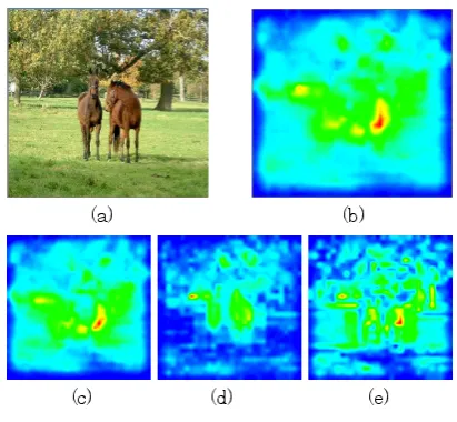
[image:4.595.328.534.52.242.2]As a method to search for visual attentional points in an image, features on SMs are generated from local intensity gradients, color information, and orientation selectivity. Fig. 2 depicts an SM and its feature maps as components. Salient regions are detected in order of high saliency regions with iterative processes. To avoid previous detected neighbor regions as an iterative pro-cess, a new detecting region is provided under the in-hibited conditions based on Euclidean distance among detected regions.
Figure 2. Saliency map and its feature maps as components: (a) original image, (b) saliency map, (c) orientation feature map, (d) color feature map, and (e) intensity feature map.
For the first step, an input image is converted repeat-edly to half size for downsampling using Gaussian pyra-mids. Our method creates nine scale images to repeat eight iterations. Herein, the 0-th image is the original image. The eighth image is the 1/256 downsampled im-age in the scalec∈[0,8]. Subsequently, center-surround difference values among scales are calculated in each pixel. We used center c∈2,3,4 and surrounds=c+δ
in δ ∈ 3,4 on respective corresponding pixels in each image.
The difference values show high if the brightness be-tween the center pixel is high and its surrounding pixels are low and the opposite combination. For this method, we used the following features: brightness I(c) in scale
c ∈[0,8], R(c), B(c), G(c), and Y(c) for color compo-nents, and orientationO(c, θ). These features are similar to the method presented by Fukuda et al. [18]. Therein,
O(x, y, θ) of coordinate (x, y) is integrated with I(x, y) and Gabor filterψ(x0, y0, θ) to calculate the amplitude.
Therein,hx,hy, andθrespectively denote the filter
win-dow size of x and y axes, and its angle. We set these parameters ashx=8, hy=8, θ∈0, 45, 90, and 135 deg.
Feature maps of RG and BY components are valid of red in the receptive field and invalid of green as dou-ble opposite color units. Moreover, the maps of I(c, s),
RG(c, s), andBY(c, s) show c of three types and s of two types. Completely, 24 maps are created from c,
s, and θ of four types in O(c, s, θ). The conspicuous maps of three channels are created from combinations of these feature maps. Before combining them, respec-tive feature maps are normalized using the maximum brightness value M. All pixels on the map are normal-ized for the range of [0, M]. Finally, SMs are created after combining conspicuous maps linearly.
Figure 3.Sample images of PASCAL Dataset: (a) original image and (b) GT image.
3.3
RoI Extraction
The Euclidean distance D between the attentional point (Xsm, Ysm) obtained from SMs and SIFT feature
point (Xsif t, Ysif t) is calculated as
D=
√
(Xsif t−Xsm)2+ (Ysif t−Ysm)2. (16)
From the order of the minimum of D, m fea-ture points are selected. The maximum im-age coordinate (Xmax, Ymax), the minimum image
coordinate (Xmin, Ymin), and the maximum SIFT
scale Smax are obtained from these feature points.
The rectangle in (Xmin−Smax, Ymin−Smax) and
(Xmax+Smax, Ymax+Smax) is defined to RoI.
3.4
Segmentation with GrabCut
For the initial procedure of GrabCut, a rectangular region is selected for teaching signals. The outside of the rectangle is labeled as background. All pixels are segmented using the model created from the color dis-tribution of foreground and background regions. The terminals are designated as the source and sink.
GrabCut creates graphs based on energy functionE, which is defined in advance. The optimal solution is calculated from the maximum flow – minimum cut the-orem. The edge cost of graphs is calculated based onE. For learning datasets, background and foreground pix-els are labeled respectively asOandB, which are called seeds. Finally, the input image is divided into graphs that correspond to foreground and background regions using the maximum flow – minimum cut theorem.
[image:5.595.62.269.55.147.2]The source and sink are ascertained from labels that are assigned to the foreground and background regions detected using SMs. The graph is constructed from the nodes of respective pixels in an image. The cost that is defined from the terminal nodes is minimized using the theorem. Herein, the cost of nodes increases along with the RGB values of pixels near terminal nodes. The cost of each node that represents the likelihood between the object and the background is smaller if RGB values of neighbor pixels are closer.
Figure 4. Results of SMs and attentional points.
4
Experimental
Results
using
Open Dataset
4.1
Dataset
PASCAL2011 is a large-scale dataset built by Mark et al. for establishing a standard benchmark dataset used in general object recognition [19]. This free dataset comprises 11,530 images including 27,450 objects of 20 categories. Annotated and Ground Truth (GT) images are attached for all images. This dataset is used for various studies of multiple object recognition such as Ravinovich et al. [3] and Okazaki et al. [4] because of the inclusion of multiple objects in all images. For this experiment, we selected 100 images that satisfied the following conditions.
4.2
Evaluation Criteria
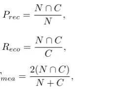
We evaluate the segmentation accuracy for Precision
Prec, Recall Reco, andF-measure Fmea as
Prec=
N∩C
N , (17)
Reco=
N∩C
C , (18)
Fmea=
2(N∩C)
N+C , (19)
whereN andCrespectively denote the number of pixels extracted as an object and the number of pixels of GT regions.
4.3
Detection
Results
of
Attentional
Points
[image:5.595.383.518.549.640.2]Table 1. Detection results of attentional points (50 images).
Num. of objects Num. of images Accuracy
Two 18 36 %
Single 27 54 %
Summation 45 90 %
0 10 20 30 40 50 60 70 80 90 100
1 2 3 4 5 6 7 8 9 10 15 20 25 30
A
cc
u
ra
cy
[%
]
Prec Reco FmeaFmea!
Reco! Prec!
Figure 5. Segmentation accuracy for 1/m.
Fig. 4(d) depicts a result of detection of single ob-jects. In Fig. 4(c), high-saliency pixels are apparent for the human walking on the snowy road. However, high-saliency regions are extended horizontally over the train in the center of the image. Attentional points were detected for the top and rear parts of the train.
Table 1 portrays detection accuracy of attentional points for 50 images. Our method detected two ob-jects from 18 images and single obob-jects from 27 images. Five images preseented failure to detect objects. For a global tendency as depicted in Fig. 4(b), valid results were obtained from the images that comprise objects to spreading horizontal and vertical directions evenly with simple background patterns. In contrast, as depicted in Fig. 4(d), attentional points were detected on a similar object for images that comprise long objects to vertical or horizontal directions with greater occupation.
4.4
Optimization of Parameters
We evaluated the following two parameters.
0 10 20 30 40 50 60 70 80 90 100
1/2 1/3 1/4 1/5 1/6 1/7 1/8 1/9 1/10
A
cc
u
ra
cy
[%
]
Prec Reco
FmeaFmea!
Reco! Prec!
Figure 6. Segmentation accuracy forn.
Figure 7. Upper two results of RoI detection and object segmen-tation.
(1) m: Number of SIFT feature points
(2) n: Number of GrabCut iterations
Fig. 5 depicts segmentation accuracy for the rate 1/m
from 1/2 to 1/10 step by 1/10. According to the decrease of m, Prec were increasing and Reca were decreasing.
Fmea obtained 56.7% as the highest at m=6. Fig. 6
depicts accuracies of nfrom 1 to 10 step by 1 and from 10 to 30 step by 5. The effect ofnwas smaller than that of m. Prec, Reca, and Fmea showed a flat curve. The
maximum accuracy ofFmeawas 57.4% atn=9.
4.5
Segmentation Results
Table 2. Segmentation accuracy for 18 images.
Image No. Prec [%] Reca [%] Fmea[%]
1 81.3 32.9 46.8
2 98.0 72.9 83.6
3 43.1 87.4 57.7
4 45.4 56.6 50.4
5 86.0 67.7 75.8
6 98.0 50.1 66.3
7 44.5 70.3 54.5
8 79.8 76.6 78.1
9 29.5 65.7 40.7
10 65.2 62.9 64.0
11 65.4 67.3 63.3
12 68.7 58.8 63.4
13 54.9 23.6 33.0
14 55.1 77.8 64.5
15 11.6 93.0 20.6
16 100.0 41.7 58.8
17 29.0 51.0 37.0
18 97.6 61.5 75.5
Average 64.1 62.1 57.4
Figure 8. Lower two results of RoI detection and object segmen-tation.
two attentional regions were detected including two ob-jects asPrec=64.1%,Reco=62.1%, andFmea=57.4%.
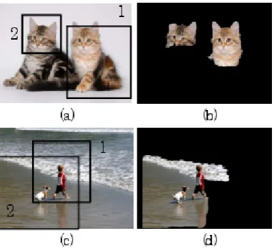
Fig. 7 depicts the top two results. Figs. 7(a) and 7(c), respectively obtained two seeps in the same cat-egory and a dog and a person in a different catcat-egory. Our method extracted RoIs including respective objects. Segmentation accuracies in Figs. 7(b) and 7(d) were, respectively, Prec=86.0%,Reco=67.7%, andFmea75.8%
and Prec=98.0%, Reco=72.9%, and Fmea=83.6%. We
obtained precision segmentation results according to ob-ject regions, althoughRecowas lower thanPrecbecause
they contain background pixels.
Fig. 8 depicts the bottom two results. Fig. 8(a) comprises a simple background of white color. The dis-tribution of SIFT feature points was sparse in the back-ground. The RoI size is smaller than the object size because feature points of the foreground were assigned to those of the background. The segmentation accu-racy in Fig. 8(b) was Prec=64.1%, Reco=62.1%, and
Fmea=57.4%. The target objects in Fig. 8(c) were a
child and a dog at a beach. Both targets are much smaller than the image size. Numerous SIFT feature points were extracted from the background region, al-though it comprises simple pattern textures with sand and surf. Therefore, the RoI size is expanded to the size of the objects. The first and second RoIs include both objects. Fig. 8(d) depicts a segmentation result that occupied the background pixels widely in the RoI. The segmentation accuracy was Prec=11.6%, Reco=93.0%,
andFmea=20.6%.
4.6
Discussion
Table 3 portrays segmentation accuracies in each object for the PASCAL dataset. The segmenta-tion accuracy of the flower category was the highest:
Fmea=60.8%. Subsequently, the house category showed
Fmea=60.0%. These objects are 1/6–1/8 compared with
those of the images. The RoIs included objects correctly. In contrast,Fmea of the car category and the cow
[image:7.595.64.265.60.243.2]cate-gory were, respectively, 26.6% and 31.8%. These objects occupied 1/4–1/2 for the images. The RoIs were smaller
Table 3. Segmentation accuracy in each category of the PASCAL Dataset.
Category Prec[%] Reco[%] Fmea[%]
Flower 99.0 43.9 60.8
House 69.4 57.3 60.0
Seep 73.7 48.7 57.2
Cat 71.0 57.5 56.9
Human 56.9 59.0 53.3
Bike 78.7 39.9 53.0
Dog 45.5 86.3 47.2
Bird 47.5 44.7 40.1
Cow 36.6 29.1 31.8
[image:7.595.322.513.91.232.2]Car 50.0 18.2 26.6
Table 4. Development and simulation tools.
Model Development tool Clock Sequential Visual Studio 2008++ 2.34 GHz
Parallel Visual Plugin 130 MHz
than the objects.
5
Parallel Implementation
5.1
Simulation Results
We evaluated the performance of our model compared with a sequential model. Table 4 portrays the develop-ment and simulation tools of the sequential model and our model. We measured the processing time of the sequential model using Visual Studio 2008. The clock frequency was 2.34 GHz, which depends on a PC. We measured the processing time of our model using VP. The clock frequency was 130 MHz, which is the maxi-mum frequency of IMAPCAR2.
We used Eclipse, an integrated software development environment, for measuring processing costs in detail because VP has no functions for it. We obtained profiles of the amount of processing time, step, and the rate for the total time.
[image:7.595.322.514.738.801.2]Table 5 depicts the processing costs for the sequential model and our model. The details are costs for creat-ing Gaussian Pyramid, intensity, color, and orientation FMs. For creating Gaussian Pyramid images, the pro-cessing costs of the sequential model and our model were, respectively, 5.2×10 ms and 1.6 ms. The processing costs in the sequential model for creating intensity, color, and orientation FMs were, respectively, 2.2×10³ ms,
Table 5. Details of processing time [ms].
Sequential Parallel Gaussian Pyramid 5.2×10 1.6
Intensity FM 2.2×10³ 18.9
Color FM 5.8×10³ 52.7
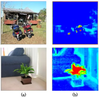
Figure 9. Results: (a) Original images and (b) SMs.
5.8×10³ms, and 1.9×10⁴ms. In contrast, the
process-ing costs in our model for creatprocess-ing respective FMs were, respectively, 18.9 ms, 52.7 ms, and 26.1 ms. The total processing costs for the sequential model and our model were, respectively, 2.7×10⁴ms and 99.3 ms. Therefore,
the processing speed of our model was 250 times higher than that of the sequential model.
For the sequential model, the processing cost for cre-ating the orientation FM was 2/3 for the total cost. In contrast, the processing cost for our model remained 1/3. To extract orientation features, kernel processing of Gabor filters entailed high processing costs. There-fore, we calculated in advance the kernel that was used for a memory table.
Fig. 9 depicts SMs for outdoor and indoor scene im-ages. For the outdoor scene image, high-saliency regions were apparent on object regions such as the number plates of the motorbikes. Similarly, for the indoor scene image, high-saliency regions were apparent on object re-gions such as the artificial flower’s leaf. We consider that SMs have effects from color features with a simple background.
Subsequently, we compare processing costs of our model with those of the method by Ouerhani et al. [14]. We converted the image resolution to 512×512 pixel. The processing costs of our model and the model by Ouerhani et al. were, respectively, 562.0 ms and 100.2 ms. This result corresponds to the 5.6 times higher speed of our model.
5.2
Hardware Setup
IMAPCAR2 is a SIMD processor developed by Rene-sas Electronics Corporation. [25]. We can create a code effectively using Visual Plugin (VP) as an integrated software developing environment and one-dimensional C (1DC) as a parallel processing programming language.
[image:8.595.345.517.54.171.2]Figs. 10 and 11 respectively show photographs of the IMAPCAR2 board and system configurations. IMAP-CAR2 is a one-dimensional combination super parallel SIMD processor, which consists of peripherals with 64 five-way VLIW 16-bit PEs, a 16-bit RISC processor for
Figure 10. Photograph of IMAPCAR2 board.
HostI/F!
Debug I/F!
Flash Download I/F!
Video capture I/F!
SV microcomputer!
Debug Host!
Program memory!
Video decoder I/C!
Video encoder I/C!
camera×2!
monitor!
EMEM I/F!
SDRAM!
IMAPCAR2
CPLD!
USB Host
IMAPCAR2 board
Figure 11. System configuration on IMAPCAR2.
a general control, a host interface, a synchronous dy-namic RAM interface, and peripheral functions such as error detection. Two USB ports are used for the bus power supply and output of video images. The SV mi-crocomputer controls operations of the whole system of the board.
Fig. 12 depicts the configuration of the IMPACAR2 board, a camera, and a scan convertor. We used a mi-cro CCD camera (Toshiba Corp.) and a scan converter (ADVC-100; Canopus Co. Ltd.). We connected the ana-log output ports of the camera and digital input ports of the board. We connected to a PC using two USB cables to display processing images directly. For this ex-periment, we took a video clip for 15 min. We used a shared space at our laboratory for an experimental en-vironment. The capture resolution was 640×240 pixels with 30 fps.
[image:8.595.320.544.224.392.2]Figure 13. Results of processing on the IMAPCAR2 board: (a), (c) input images and (b), (d) SMs.
5.3
Performance Evaluation
For this implementation, the mean processing time was 47.5 ms, which corresponds to 21.1 fps. Fig. 13 portrays two sample results. High-saliency regions were apparent around object regions such as the chairs and the bookshelves. Comparison with the results obtained using the PASCAL dataset, high-saliency regions were apparent on small objects of various types. We infer that this tendency results from the number of objects in these images.
2!
3!
4!
5!
6!
7!
8!
9!10!
D
oor
!
W
in
dow
!
C
h
a
ir
!
"
C
h
a
ir
!
C
h
a
ir
!
C
a
b
in
et
!
Desk!
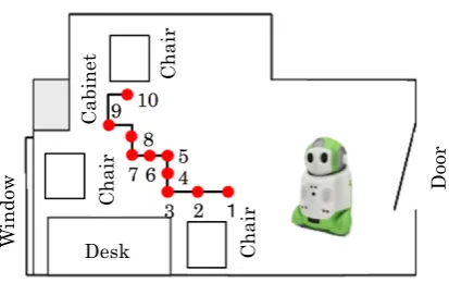
[image:9.595.315.524.55.150.2]Figure 14. Room layout, route, and robot used for this experi-ment.
Figure 15. Image obtained for position 2 and its saliency map.
6
Application to Robot Vision
6.1
Experimental Setup
For application in an actual environment and ad-vanced performance evaluation, we conducted segmenta-tion used for time-series images obtained using a mobile robot. We used PaPeRo developed by NEC Corp. The body is 385 mm high, 282 mm long, and and 251 mm wide. This robot has sufficient capabilities to move on the floor at 23 cm/s maximum. Moreover, servomotors are used for the drive system to control movements with high precision. Two cameras are mounted for stereo vi-sion. We used a single camera for monocular vision. The specifications of the cameras are: imaging device, 1/4 inch CCD; image format, motion JPEG; and reso-lution, 320×240 pixel.
Fig. 14 depicts the layout of the experimental environ-ment. This is a vacant room used as a professor’s room at our university. It contains a desk, a table, a cabinet, and chairs. We used them for detection and segmenta-tion targets. In the room are a window and a blind. We closed the blind to avoid effects of sunlight while taking images through the experiment. We set two objects as segmentation targets from each image that are similar to the former section. We used ten images taken at ten points. The circles in Fig. 14 correspond to the points. The numbers correspond to the image obtained position. Fig. 15(a) depicts an image obtained at position 2. We created GT mask images manually using a drawing tool.
6.2
Segmentation Results
Fig. 15(b) depicts that high-saliency regions were ap-parent on the chair back and the left part of the table. Fig. 16(a) depicts a RoI extraction result for the im-age of Fig. 15(a). For ten imim-ages, RoIs that included two objects were extracted from seven images. From the other three images, only single objects were extracted.
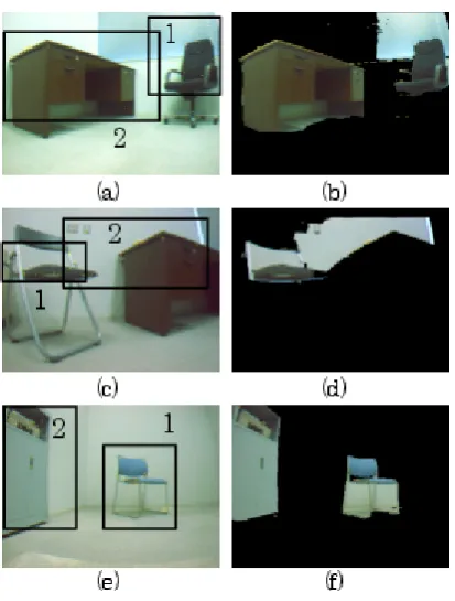
Subsequently, we applied our method for the seven images above. Fig. 16 depicts typical segmentation results. Fig. 16(b) obtained the highest accuracy:
Prec=68.9%, Reco=94.0%, andFmea=79.6%. The RoIs
in Fig. 16(c) obtained merely a part of the chair and the desk. The second RoI extended to the left size that included the background region between the table and a part of the chair back. Therefore, our method extracted background pixels to foreground pixels. The segmen-tation accuracy dropped dramatically to Prec=21.3%,
Reco=11.4%, andFmea=14.9%. Both RoIs in Fig. 16(e)
[image:9.595.61.268.642.772.2]Figure 16. RoI extraction results and segmentation results.
Table 6. Segmentation accuracy in each category of our original dataset.
Category Prec [%] Reco [%] Fmea [%]
Desk 42.0 77.6 51.4
Chair 51.9 67.1 50.5
Cabinet 65.9 28.5 35.8
the first RoI extracted not only the chair back, but also the chair legs. Prec in Fig. 16(f) was 78.6% because
both chair and cabinet were extracted correctly. How-ever,FmeaandRecowere, respectively, 33.3% and 46.7%
because background pixels near the chair legs were ex-tracted. The mean segmentation accuracy for seven im-ages wasPrec=58.0%,Reco=63.1%, andFmea=58.1%.
6.3
Discussion
Table 6 portrays segmentation accuracies in each ob-ject of our original dataset. The segmentation accura-cies ofFmeawere 50.5%, 51.4%, and 35.8%, respectively,
[image:10.595.74.281.686.779.2]for the chairs, the table, and the cabinet. SIFT feature
Figure 17. Result of detected three RoIs.
points were apparent for the video recorder that is lo-cated inside the cabinet. SIFT feature points were not extracted from the overall cabinet. This is our future work to improve our method for overlapped objects.
Numerous objects exist in our actual environment. For the application to robot vision, several images con-tain three objects. Fig. 17 depicts a result to increase the iterations of RoI extraction for three times. Fig. 17(a) depicts a SM that contains three high-saliency parts. Fig. 17(b) depicts RoI extraction results. The RoIs respectively included the cabinet, the desk, and the chair for this priority. The first and second RoI respectively extended the right side and left side, al-though both RoIs were not overlapped. Therefore, the third RoI was used for the overlapping region of the first and second RoIs. The number of SIFT feature points was decreased for an image consisting of simple back-ground patterns. For detection of three objects, RoIs were overlapped to other images. In contrast, Fmea of
three-object segmentation was higher than that of two-object segmentation because of the expansion of two-object regions. We infer that our method can be extended to multiple object segmentation of more than two objects.
7
Conclusion
This paper presented a segmentation method com-bined with SMs and GrabCut. Our method achieved ex-traction of multiple objects without learning in advance. We applied our method to the PASCAL2011 dataset for extraction of objects in 100 images. Attentional points were extracted correctly from 18 images for two ob-jects and from 25 images for a single object. The mean segmentation accuracies werePrec=64.1%,Reco=62.1%,
andFmea=57.4%. For the implemented experiment, the
processing cost was 47.5 ms for an image with 640×240 pixel resolution. Moreover, we applied our method to time-series images obtained using a mobile robot. Atten-tional points were extracted correctly for seven images for two object and three images for single objects from ten images. The mean segmentation accuracies were
Prec=58.0%,Reco=63.1%, andFmea=58.1%. These
ex-perimentally obtained results present the possibility of applying our method used in an actual environment of our life.
Our future work is to modify our method to learn time-series features and to evaluate the robustness of appearance changes of objects. Moreover, we would like to apply our method to multiple object recognition to increase the number of possible target objects.
REFERENCES
[1] K, Yanai, “The Current State and Future Directions on Generic Object Recognition,” IPSJ Computer Vision and Image Media, vol.48, pp.1–24, 2007.
[3] A. Rabinovich, A. Vedaldi, C. Galleguillos, E. Wiewiora, and S. Belongie, “Objects in Context,”Proc. IEEE International Conference Computer Vision, pp.1– 8, 2007.
[4] T. Inamura, M. Inaba, and H. Inoue, “Incremental Ac-quisition of Behavior Decision Model based on Inter-action between Human and Robots,” Journal of the Robotics Society of Japan, vol.19, no.8, pp.983–990, 2001.
[5] D. Das, Y. Kobayashi, and Y. Kuno, “Multiple Object Category Detection and Localization Using Generative and Discriminative Models”,IEICE Trans. Information and Systems, vol.E92–D, no.10, pp.2112–2121, 2009.
[6] L. Itti, C. Koch and E. Niebur, “A Model of Saliency-Based Visual Attention for Rapid Scene Analysis,” IEEE Trans. Pattern Analysis and Machine Intelli-gence, vol.20, no.11, pp.1254–1259, 1998.
[7] T. Liu, “Learning to Detect a Salient Object,” IEEE Trans. Pattern Analysis and Machine Intelligence, vol.33, no.2, pp.353–367, Feb. 2011
[8] T. Fujisaki and S. Inoue, “Automatic Object Extraction Using graph cuts with Visual Attention Cues,” Techni-cal Report of IEICE. PRMU, vol.108, no.432, pp.145– 150, 2009.
[9] K. Fukuchi, K. Miyazato, A. Kimura, S. Takagi, and J. Yamato, “Saliency-based video segmentation with graph cuts and sequentially-updated priors,” Proc. International Conference on Multimedia and Expo, pp.638–641, 2009.
[10] V. Pham, K. Takahashi, and T. Naemura, “Bounding-box based Segmentation with Single Min-Cut using Dis-tant Pixel Similarity,”Proc. 20th International Confer-ence on Pattern Recognition, pp.4420–4423, 2010.
[11] V. Pham, K. Takahashi, and T. Naemura, “Image Seg-mentation from Bounding Shape without Using Ap-pearance Model,” IEICE Trans. Information and Sys-tems, vol.J94–D, no.8, pp.1183–1193, 2011.
[12] C. Rother, V. Kolmogorov, and A. Blake, “GrabCut – Interactive Foreground Extraction using Iterated Graph Cuts,”ACM Trans. Graphics, vol.23, no.3, pp.309–314, 2004.
[13] N. Kapre, D. Walther, C. Koch, and A. DeHon, “Saliency on a chip,” The Neuromorphic Engineer, 2004.
[14] N. Ouerhani, H. Hugli, P. Burgi, and P. Ruedi, “A Real Time Implementation of the Saliency-Based Model of Visual Attention on a SIMD Architecture,”Pattern Recognition, vol.2449, pp.282–289, 2002.
[15] A. Yamanashi, H. Madokoro, Y. Ishioka, and K. Sato, “Visual Saliency Based Segmentation of Multiple Ob-jects Using Variable Regions of Interest,” Proc. 14th International Conference on Control, Automation and Systems, pp.1046–1051, 2014.
[16] K. Shirai, H. Madokoro, S. Takahashi, and K. Sato, “Parallel Implementation of Saliency Maps for Real-Time Robot Vision,”Proc. 14th International Confer-ence on Control, Automation and Systems, pp.88–93, 2014.
[17] P. Ruedi, P Marchal, and X. Arreguit, “A Mixed Digital-Analog SIMD Chip Tailored for Image Percep-tion,” Proc. International Conference on Image Pro-cessing, vol.3, pp.1011–1014, 1996.
[18] K. Fukuda, T. Takiguchi, and Y. Ariki, “Automatic Segmentation Using graph cuts Based on AdaBoost and Saliency Map,” Proc. Meeting on Image Recognition and Understanding, pp.796–801, 2008.
[19] M. Everingham, L. Gool, C. I. Williams, J. Winn, A. Zisserman, C. Williams, and J. Winn, “The PASCAL Visual Object Classes Challenge,” International Jour-nal of Computer Vision, vol.88, no.2, pp.303–338, 2009.
[20] H. Madokoro, Y. Utsumi, and K. Sato, “Unsupervised Indoor Scene Classification Based on Context for a Mobile Robot,” Journal of Robotics Society of Japan, vol.31, no.9, pp.918–927, 2013.
[21] Y. Ishioka, H. Madokoro, and K. Sato, “Automatic Ex-traction Method of Object Regions Based on Visual Salience for Multiple Object Recognition,”Proc. Meet-ing on Image Recognition and UnderstandMeet-ing, 2012.
[22] Y. Fujita, “Childcare Robot PaPeRo,” Journal of Robotics Society of Japan, vol.24, no.2, pp.162–163, 2006.
[23] T. Lee, “Image Representation Using 2D Gabor Wavelets,”IEEE Trans. Pattern Analysis and Machine Intelligence, vol.18, no.10, pp.959–971, 1996.
[24] M. Everingham, L. Gool, C. I. Williams, J. Winn, A. Zisserman, C. Williams, and J. Winn, “The PASCAL Visual Object Classes Challenge,” International Jour-nal of Computer Vision, vol.88, no.2, pp.303–338, 2009.
[25] S. Kyo, “Image Recognition Using the SIMD/MIMD Dynamic Mode Switching Processor,” The Journal of the Institute of Electronics, Information, and Commu-nication Engineers, vol.94, no.6, pp.464–469, 2011.