Measuring the Economic and Environmental Impacts of Using Shale Oil and Gas Resources: A Computable General Equilibrium Modeling Approach

Measuring the Economic and Environmental Impacts of

Using Shale Oil and Gas Resources: A Computable

General Equilibrium Modeling Approach

Farzad Taheripour

_{, Wallace E. Tyner}

Department of Agricultural Economics, Purdue University, USA

Copyright © 2015 by authors, all rights reserved. Authors agree that this article remains permanently open access under the terms of the Creative Commons Attribution License 4.0 International License

Abstract

have increased significantly recently and are expected to continue to grow in the future. Using these resources generates significant economic benefits for the US economy. Interestingly, prior to 2007, except for those in the industry, shale resources were not at all part of the picture. Thus, it is reasonable to consider the economic benefits of shale as a sort of dividend. This paper first quantifies the shale dividend for the US economy and then asks how much of the dividend would we have to give up to achieve significant GHG reductions defined in the President Obama’s Clean Energy Standard (CES) and the Corporate Average Fuel Economy (CAFE) policies. We modify and use a well-known computational general equilibrium model to accomplish these tasks. Our results confirm that the shale technology is a game changer for the US economy yielding annual benefits between 2008 and 2035 averaging $302 billion per year relative to 2007. We also estimated the costs for the US economy of implementing the CES and CAFE jointly. These two policies jointly reduce the shale dividend from $302 billion per year to $148 billion per year on average. In other words, the shale economic gains can be used to pays the cost of emissions reduction.

Keywords

Gains, General Equilibrium, US Emission Reduction Policies

1. Introduction

Recent improvements in hydraulic fracturing (fracking) and horizontal drilling technologies have increased access to more unconventional oil and gas resources. These resources (including: shale and tight oil and gas) are trapped in shale formations and sandstone. Until very recent improvements in fracking and horizontal drilling technologies in the US, unconventional oil and gas resources were mainly inaccessible, except for some limited activities. The

unconventional resources are found all across the world. According to the existing estimates, about 335 billion barrels of crude oil and 221 trillion cubic meters of natural gas can be extracted from shale resources at the global scale. The corresponding estimates for US are 48 billion barrels of crude oil and 32.9 trillion cubic meters of natural gas [1]. In recent years, the US supplies of oil and gas have increased significantly from shale resources due to improvements in fracking and horizontal drilling technologies. The US Department of Energy projections indicate that producing energy from shale resources will continue to grow in decades to come [2]. These projections suggest that by 2030 North America will be self-sufficient in petroleum. Currently, the US is the only country which extracts oil and gas from shale resources to any significant degree. Extracting these resources in the US will have major economic and environmental consequences for the global economy, altering the energy market at the global scale. The economic benefits from shale resources also could provide new opportunity to pursue emissions reduction polices in the US1_.

The existing literature indicates that some studies have evaluated the economic gains due to expansion in producing shale gas, and some others have examined the costs of emission reduction polices in the presence of expansion in shale gas. However, to the best of our knowledge no one has examined the economic gains due to producing more oil and gas from shale resources in the absence and presence of emission reduction polices.

This paper aims to evaluate the economic gains of using shale resources for the US economy. It then asks the question of the relative size of the economic gains from shale oil and gas compared with the economic costs that would be incurred if the US were to also launch aggressive CO2

emission reduction policies. Among alternative modeling

1 Shale oil and gas technology has been controversial due to direct environmental impacts in the shale producing areas. We believe that the direct environmental issues associated with fracking are important, and must be dealt with in the regulatory structure. However, that is not the subject of this paper.

approaches that can be used to answer these questions, given the economy wide impacts of using shale resources, a global Computable General Equilibrium (CGE) model can provide more reliable and comprehensive results. Hence, we used a modified version of a well-known global CGE model (GTAP-E, introduced in the modeling section) to achieve the goals of this paper. Since the original GTAP-E model and its data base do not cover shale oil and gas resources, as mentioned in the modeling section, we made several changes in this model to be able to conduct this research. Using the modified GTAP-E model we showed that producing more oil and gas from shale resource generates major economic gains for the US economy in the absence of any emission reduction policy. Then we showed that a carbon tax which reduces the US carbon emissions in by 27% in 2035 compared to 2007 would lead to economic losses of about 40% of the economic gains due to the expansion in shale oil and gas production.

In what follows, we first provide a brief review of the limited literature to date on the economic and environmental impacts of shale oil and gas development. Then we introduce the model and data base modifications we have done in GTAP-E to permit simulations of the shale oil and gas impacts. After that we introduce our experiments which were designed to examine the economic impacts of producing oil and gas from the shale resources in the absence and presence of emissions reduction policies. Finally, we analyze our simulation results and provide some conclusions.

2. Literature Review

Recently, a limited number of studies have tried to quantify the economic and environmental consequences of the new developments in the US energy market. The existing literature in this field can be divided into two categories. The first category mainly inspects the links between producing more shale gas with US emission reduction polices. The second group tries to measure the economic gains due to producing more gas from shale resources in the US.

The expansion in US gas production from shale resources provides an opportunity for the US economy to move away from coal (a very dirty source of energy) and use more gas (a cleaner source of energy). However, the extent to which this shift may occur in the real world will depend on future emissions reduction policies. Several papers have examined this topic. These papers usually do not take into account future growth in production of oil from shale resources. We review three main papers from this group. Brown et al. [3] have examined several energy and climate policy scenarios using an energy-economy market equilibrium model and concluded that the growth in supply of natural gas from shale resources in combination with carbon polices could support the US economy to achieve low-carbon standards in future. Paltsev et al. [4] have studied the growth in the US natural gas production from shale resource as well. These authors have focused on the trade, production and use of natural gas in future decades. They used two CGE models and showed that even in the absence of additional GHG abatement

policies, production and use of gas in 2050 will be higher than today and that shale gas will help to achieve a lower level of emissions. Jacoby et al. [5] also examined the impacts of the expansion in US shale gas on US energy and environmental policy and reached similar conclusions.

In an early research in this area the IHS Global Insight Inc. [6] projected the economic impacts of the expansion in supply of gas for the US economy until 2035 using a macroeconomic model of the US economy in combination with an industry model. This research projected that about $1.9 trillion will be invested in shale gas during the time period of 2010-35. They also projected that the growth in shale gas industry will add 0.9 million and 1.6 million job opportunities in the US in these years. The simulation results obtained from this research show that the growth in shale gas will increase the US GDP by $118 billion and $231 billion in 2015 and 2035, respectively. In a different paper the Citi GPS [7] has also estimated the gains due to growth in shale gas in the near future in the US. Again using a US macro model this research concluded that the growth in gas supply could improve the US GDP up to 3% in 2020. Arora [8] using a US macro CGE model concluded that the expansion in supply of natural gas will improve the US GDP by a small to moderate rate with a full employment assumption. Sarica and Tyner [9] used a hybrid model named MARKAL-Macro to evaluate the impacts of a carbon tax and other policies on the US energy mix as well as economic impacts on the economy. They find that a policy such as the clean energy standard proposed by President Obama and the Corporate Average Fuel Economy (CAFE) rules would substantially change the energy source mix in the electricity sector by 2035 with coal being largely displaced by natural gas, wind energy, and other sources. They also find that such an emission reduction policy would lead to a 1-2% GDP reduction depending on how it was implemented.

While these papers provided important analyses on the impacts of the expansion in shale gas, they missed the impacts of simultaneous growths in both shale oil and gas. They ignored the interaction between economic gains and environmental policies in the presence of expansion in using shale resources. In a recent study, Taheripour et al. [10] using a modified version of the GTAP-E model evaluated the economic gains due to increases in oil and gas production from shale resources for the US economy until 2035. Henceforth we refer to this paper as TTS. These authors developed scenarios with and without expansion in using shale resources and showed that the US GDP on average would be 2.2% higher during the time period of 2008-35 compared with its original level in 2007. These authors also have shown that with no regulation in place, producing more oil and gas from shale resources could increase US total CO2

emissions. Like other papers in this area, these authors also did not take into account the possible interaction between economic gains and environmental policies in the presence of expansion in using shale resources.

the economic impacts of expansion in using shale resources. The existing literature confirms that in the presence of proper emissions reduction policies, the expansion in US gas production from shale resources can help the US economy to produce fewer emissions in future. On the other hand, the existing estimates indicate that producing more oil and gas from shale resources generates significant economic gains for the US economy. It is also common knowledge that the emissions reduction polices are not free and generate some welfare losses. Thus, the country is clearly presented with an economic gain from shale resources, and the opportunity to use part of that gain if we choose to reduce greenhouse gas (GHG) emissions. Hence, the question that we try to answer in this paper is: What are the relative magnitudes of the shale benefits and the economic costs of GHG reduction? We find that half or less of the shale dividend would be required to achieve the GHG reduction.

3. Methods

3.1. Modeling Background

To capture the economy-wide impacts of using shale oil and gas resources, we extensively modified and used an advanced version of the standard GTAP model developed by Hertel [11]. This is a well-known global CGE model which has been broadly used in a wide range of research on

economic, environmental, and energy topics. GTAP traces production, consumption, and trade of a wide range of goods and services at a global scale and by region. As represented in Figure 1, in this model in each country (e.g., USA) a regional household collects all the regional incomes and spends those over three expenditure categories: private household (consumer), government, and savings. The model determines the household and government demands for goods and services and traces saving and investment in each region and at the global scale. The model divides economic activities into several sectors. In each sector a representative firm maximizes profits subject to a production function that combines primary factors and intermediate inputs to produce a final good. Firms pay wages/rental rates to the regional household in return for the employment of land, labor, capital, and natural resources. On the other hand, firms sell their output to other firms (as intermediate inputs), private households, government, and investment. Since this is a global model, firms also export the tradable commodities and import the intermediate inputs from other regions. These goods are assumed to be differentiated by region, so the model can track bilateral trade flows. The rest of the world gets revenues by exporting to private households, firms and government. This rest of world composite is actually made up of many other regions. The supply and demand functions along with market clearing conditions and other relationships implemented in this model are presented in Hertel [11].

GTAP-E, a special version of the standard GTAP, provides a comprehensive framework to examine the sectoral and economy wide consequences of changes in markets for energy sources and products (such as crude oil, gas, coal, refined petroleum products, and electricity) and/or emissions reduction, energy, and trade policies. Burniaux and Truong [12] and McDougall and Golub [13] outlined the details of this model.

To evaluate the economic impacts of expansion in production of oil and gas from shale resources we made major changes in the GTAP-E model and its data base. TTS briefly introduced some of these modifications. In this section we document those modifications in greater detail. We made some changes in the model to examine the interactions between the US emissions reduction policies and the expansion in production of oil and gas from shale resources. These model modifications are also introduced in this section.

3.2. Modifications in GTAP-E Model and its Data Base 3.2.1. Data base modifications

The GTAP data base version 8 [17], which represents the world economy in 2007 (classified into 129 countries/regions and 57 commodities) is used in this paper. This data set includes regional input-output tables along with comprehensive data on trade, energy production and consumption, and greenhouse gas emissions. The following major corrections and modifications were made in this data base to make the data base more consistent with real world observations: 1) Biofuels were added to the data base; 2) Regional monetary values of gas production and consumption and of gas purchased by the gas distribution sector were corrected; 3) Natural resources were divided into different categories.

The standard GTAP data bases do not explicitly represent production, consumption and trade of biofuels. Given that several countries were producing large amounts of biofuels in 2007, following Taheripour et al. [14], we introduced production, consumption, and trade of biofuels including ethanol produced from food grains and sugarcane and biodiesel produced from oilseeds into the GTAP data base. This is an important modification because it allows us to capture the interplays between biofuels and fossil fuels (including oil and gas produced from shale resources) in the presence of emission reduction polices in our experiments.

Based upon careful examination of the detailed GTAP data base, we learned that it under estimates the regional monetary values of gas production and consumption and of gas purchased by the gas distribution sector (“gdt”) as explained in detail in Appendix A. Since expansion in using shale resources will increase the supply of gas and its consumption, we fixed these issues to provide more accurate estimates of monetary values of future expansion in supply of gas, as explained in Appendix A.

The last data base modification divides the payments to

natural resources into 5 different categories. This is a simple, but very important modification for this research. The standard GTAP data base defines a common pool of natural resources, and producers share the pool. Then the standard GTAP model considers natural resources as a sluggish endowment with limited movement across sectors. We altered this set up to model the expansion in oil and gas reserves due to improvements in fracking and horizontal drilling technologies and define sector specific resources as explained in the next section. To accomplish this task we divided natural resources into 5 different groups of natural resources including fishery, coal, oil, gas, and other resources.

3.2.2. Model Modifications: Revising firms’ demand nesting structure

The GTAP-E model uses nested constant elasticity of substitution production functions to represent firms’ behavior and determine their demands for intermediate and primary inputs including capital, labor, land, and resources as shown in Figure 2. At the very bottom of this production tree, firms bundle crude oil, natural gas, and petroleum products with the substitution elasticity of σ_ELNCOAL to create non-coal energy sources. At the higher level the non-coal and coal items are combined with the substitution elasticity of σ_ELNEL to generate non-electricity energy sources. At a higher level, electricity and non-electricity items are combined with the substitution elasticity of σELEN to form the

composite of all energy items under one category. Then at one level higher capital and energy are combined to allow substitution between these items with the elasticity of σELKE.

At the next higher level, primary inputs such as land, labor, and resources are mixed to obtain the composite of value added and energy with the substitution elasticity of σESUBVA.

Finally, at the highest level of the tree the mix of value added and energy is combined with the mix of other intermediate inputs with the substitution elasticity of σESUBT to produce

the final product. As shown in Figure 2, the energy and non-energy intermediate inputs can be obtained either from domestic or foreign markets.

structure is presented in Figure 3. At the very bottom nest, biofuels are introduced in the nest. Then unlike the original model coal and gas are mixed directly to represent the direct substitution between gas and coal. Then at a higher level the combination of coal-gas substitutes with oil and petroleum products to generate the non-electricity energy input. From this point to the top production function we preserved the original GTAP-E nesting structure.

The production functions associated with the original and modified nesting strictures presented in figures 2 and 3 are shown in Appendix B. The first table of this appendix represents the Constant Elasticity of Substitution (CES) production functions used in the original GTAP-E model, and the second table demonstrates the modified CES production functions.

Figure 3. Modified GTAP-E Production Nesting Structure

3.2.3. Model Modifications: Other Major Modifications in GTAP-E model

The GTAP-E model and its data base do not distinguish between alternative natural resources and bundle all types of natural resources under one category. We altered this set up and distinguished between fossil fuels and other resources to model the expansion in shale resources. Then we used the information developed by the US Department of Energy [2] to determine the magnitudes of the expansions in these resources over time.

emitters in the US with 40 and 34 percent of total emissions respectively [16]. Thus it is understandable that these sectors would be targeted by current US policy. The combined goal of the regulatory policies (including the average fleet efficiency (CAFE) standard, renewable fuel standard (RFS), and clean energy standard (CES) for electricity is to reduce CO2 emissions in 2035 by 27%, compared to 2007 (Sarica

and Tyner, 2013). We altered the GTAP-E model to examine the joint impacts of reductions in emissions generated by the transportation and electricity sectors.

Finally, the original GTAP-E model assumes that all primary factors of production including labor, land, capital, and natural resources are fully employed in the short run. This is not a plausible assumption for a relatively long time period, as using shale resources affects the labor market in the long run. Therefore, unlike the GTAP-E model, we assumed that supplies of labor and capital grow as the production of oil and gas from shale resources expand. We tuned the supply elasticities of labor and capital according the numerical results reported in Citi GPS [7].

3.3. Designed Experiments

To achieve the goals of this paper, we developed the following four experiments/cases:

Case 1: Expansion in supplies of oil and gas produced from shale resources with no carbon emission reduction

policy in place. This experiment is designed to capture the

economic impacts of producing more oil and gas from shale resources, while we assume that the government does not control emissions. In this experiment we shock production of oil and gas (induced by technological progress in these sectors) according to the DOE projections for oil and gas produced from shale resources in 2007-2035. Given these shocks our model projects changes in the endogenous economic variables compared with the base year (2007).

Case 2: Expansion in supplies of oil and gas produced from shale resources with a uniform economy-wide carbon

tax to cut emissions by 27% compared to 2007. In this

experiment we repeat the first experiment while we assume that the government imposes a non-discriminatory uniform emissions tax across all sectors, commodities, and sources of emissions to reduce emissions by 27% compared to the base year. Therefore, in this simulation two forces determined the results: 1) increases in oil and gas production from shale resources compared to the base year and 2) a uniform emissions reduction policy to reduce emissions by 27% again compared to the base year (2007).

Notice that the emissions reduction policy which we used in this experiment is usually referred to as the least cost emissions reduction policy. However, currently the US does not pursue this policy to reduce GHGs emissions. Instead, the US concentrates on CAFE, RFS, and CES policies to reduce emissions. The next experiment represents the impacts of these policies.

Case 3: Expansion in supplies of oil and gas produced from shale resources with a carbon tax imposed only on

electricity and transportation sectors to cut emissions by

27% compared to 2007. This experiment is similar to the

second experiment, but instead of using a uniform economy-wide emission tax, imposes the emission tax only on the electricity and transportation sectors to achieve the 27% emission reduction targets. The implemented policy in this experiment represents the joint impacts of CAFE, RFS, and CES policies.

Case 4: Expansion in supplies of oil and gas produced from shale resources with a carbon tax imposed only on

electricity sector to cut emissions by 27% compared to 2007.

This experiment is similar to the third one, but transportation is the only sector which bears the burden of the emission tax.

All of the above experiments consider a goal of 27% reduction in carbon emissions for the US. To examine the sensitivity of the results with respect to this target we repeated the second experiment (i.e. case 2) under several emissions reduction targets, from 0% to 60% in 15% increments. The next section presents the results.

4. Results

To concentrate on the economic gains of producing more oil and gas from shale resources under alternative emission reduction scenarios, we only report the average results for 2008-2035 compared with the base year (2007).

4.1. Case 1 – Shale Expansion Only

The first block of Table 1 provides the percentage change in output, prices, and trade balance for major US commodity groups for case 1. As would be expected, the biggest changes are in output, prices, and trade of oil and gas. Oil and gas production are expected to increase 31% and 39%, respectively. Their prices fall 8% and 12% correspondingly. With no emission reduction policy in place, the growth in gas and oil production leads to a negligible reduction in coal production (1.4%). This means that with no emission reduction policy, the US economy only reduces coal production by a small amount due to expansion in using shale resources. Indeed, the negative impact on coal demand due to substitution of cheap oil and gas is counterbalanced by the positive impact of increased income, which increases the demand for energy. As shown in the next section, production of coal drops significantly in the presence of emissions reduction policies.

Table 1. Selected Key Simulation Results for Cases 1 and 2

Sector Case 1 Case 2

Outputs %Change Prices %Change Trade Balance _{Million Dollar} Outputs %Change Prices %Change Trade Balance _{Million Dollar} Crops 0.16 2.9 -1,414 -0.36 0.96 -998 Livestock 1.46 0.67 -228 0.64 0.71 -172 Forestry 0.98 0.89 -62 -0.10 0.47 -20

Fishing 0.76 1.20 -68 0.03 1.26 -49 Food 1.63 0.44 -3,234 0.77 0.65 -2,935 Coal -1.40 0.27 -182 -35.14 -4.68 912

Oil 30.80 -7.82 20,703 30.80 -10.12 40,103 Gas 38.90 -11.70 32,811 38.90 -13.28 42,019 Gas Distribution 9.43 -6.83 297 2.20 -6.50 769

Oil Products 5.62 -3.56 2,890 0.69 -3.86 6,563 Biodiesel 5.29 0.59 0 -1.09 0.97 0

Ethanol 5.29 0.30 0 -1.09 2.01 0 Electricity 2.36 -1.28 -6 -4.61 8.97 -1,082 Chemical Ind. 0.81 -0.02 -8,303 -1.17 0.56 -11,244 Energy Intensive Ind. 0.70 0.01 -3,506 -2.18 1.15 -6,488

Other Industries 1.26 0.43 -65,494 -0.40 0.55 -42,786 Transportation 2.52 -0.75 -1,202 -0.36 1.82 -6,822

Services 2.05 0.64 -15,523 1.19 0.54 -9,778 Source: Simulation results obtained from case 1. Each figure represents average change for the time period of 2008-2035 compared with the base year of 2007.

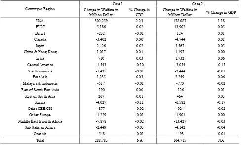
Table 2. Key Economy-Wide Simulation Results for Cases 1 and 2

Country or Region _{Change in Welfare in} Case 1 Case 2

The first block of Table 2 provides the changes in welfare (measured in terms of Equivalent Variation 2 (EV)) and GDP by region for case 1. This block shows that in the absence of environmental regulation, producing more oil and gas from shale resources improves US welfare by more than $300 billion per year relative to the 2007 level. Similarly US GDP increases, on average by 2.2% compared with 2007. The main regions negatively impacted by the expansion in using US shale resource are the Middle East and Russia – major oil and gas exporters. Canada, also an oil exporting county, suffers from higher US production. The European Union is positively impacted. In total, the US shale oil and gas expansion reduces welfare by about $14 billion in all of the rest of world, a very small amount. So the bulk of the impact of the US shale oil and gas expansion is within the US. Finally, the first block of Table 1 indicates that producing more oil and gas from shale resources in US barley affects GDP of other countries. Of course some countries gain and some loss.

4.2. Case 2 – Shale Expansion Plus a Uniform Economy Wide Carbon Tax

As shown in the second block of Table 2 in case 2, when we add the economy wide uniform carbon tax, the welfare gains for the US drop to $178 billion, a drop of 41% compared with the welfare gains of case 1. The GDP level increase falls from 2.2 to 1.2% as well. This may seem like a large loss, but it is a glass half empty or glass half full question. Yes, 41% of the shale gain is lost, but substantial reduction in GHG emissions has been achieved. While we do not have quantitative estimates of the benefits of avoiding the adverse impacts of climate change, they clearly cannot be ignored. Another way to interpret these results is that we can at the same time have more fossil energy and achieve substantial economic gains, while also reducing GHG emissions 27% from the 2007 base. As shown the second block of Table 2, imposing an emission reduction policy in the US decreases welfares of oil exporting regions (Middle East & North Africa and Russia) and also Canada significantly, due to lower emission intensity. In this case the European Union gains more, due to lower emission intensity.

The second block of Table 1 represents changes in US outputs, prices, and commodity trade balances for case 2. The important differences between these results and case 1 are as follows:

 Coal output drops by 1.4% in case 1, and it falls by 35.1% in the carbon tax case. This means that production of coal goes down significantly in the presence of the carbon tax. This result is consistent with prior research on the carbon tax [9], using a completely different modeling framework. The

2 In general, in a CGE modeling framework usually EV measures changes in consumers’ and producers’ surpluses due to changes in policy variables (such as tax) and/or changes in exogenous variables (such as technological progress). The GTAP model includes a module which calculates EV. For more information see Huff et al. [18]

simulation results also show that in the presence of emissions reduction policy, the US even exports a portion of its coal production to other countries as well. On average the net trade of coal increases by $912 million in the presence of the carbon tax.

 Trade balances for oil, gas, and petroleum products improve to $40 billion, $42 billion, and $6.6 billion, due to reduction in US fuel consumption with the carbon tax.

 Electricity output increases 2.4% in case 1, but falls 4.6% with the carbon tax

 While all the industrial sectors grew in the shale expansion case, they all contract a bit in the carbon tax case.

 Coal price was relatively flat in the shale expansion case but falls 4.7% with the carbon tax.

 Electricity price drops by 1.3% in case 1 but increases 9% with the carbon tax.

 The industrial trade balance improves relative to the shale expansion case because incomes are not rising as much.

4.3. Case 3 – Shale Expansion Plus Carbon Tax Imposed Only on Electricity and Transportation

In case 3 we consider an option that approximates current US energy policy; that is, expansion of shale oil and gas resources along with regulations on electricity and transport emissions that together achieve the 27% reduction in emissions. In essence, this policy concentrates all the emission reduction in the two sectors that together represent 71% of all GHG emissions. With this policy, as shown in the first block of Table 4, the US welfare gain falls from $302 billion in case 1 and $178 billion in case 2 to $148 billion. Cases 1 and 2 had GDP gains of 2.2 and 1.2%, whereas case 3 has a gain of 1%, as shown in the first block of Table 4. The US welfare gain in case 3 is $30 billion less than the gain from case 2. This indicates that by avoiding the more efficient economy-wide carbon tax and instead using regulatory measures to achieve the same objective, the welfare cost to the economy is about $30 billion/year.

The first block of Table 3 represents changes in outputs, prices, and trade balances for case 3. The main differences compared to the first two cases are as follows:

 Coal output falls even further to -39%. This difference is to be expected since more of the emission reduction is forced on the electricity sector and that reduces coal production and consumption by large quantities. US net coal exports increase from $912 million in case 2 to $1147 in case 3.

 All the fossil energy prices fall significantly.

 Electricity price goes up 12.5% compared with 9% in the carbon tax case.

 All the industrial prices go up more than in the carbon tax case.

 The industrial trade balance improves a bit compared with the carbon tax case.

Table 3. Selected Key Simulation Results for Cases 3 and 4

Sector Case 3 Case 4

Outputs %Change Prices %Change Trade Balance _{Million Dollar} Outputs %Change Prices %Change Trade Balance Million _Dollar Crops 0.13 1.44 -648 0.16 1.66 -671 Livestock 0.60 0.45 -126 0.75 0.31 -109 Forestry -0.15 0.35 -17 0.02 0.36 -19

Fishing 0.48 0.38 -27 0.51 0.45 -31 Food 0.70 0.42 -2,189 0.83 0.29 -1,918 Coal -38.98 -5.71 1,147 -42.60 -7.09 1,426 Oil 30.80 -9.29 33,573 30.80 -7.79 21,410 Gas 38.90 -12.14 35,638 38.90 -11.99 34,985 Gas Distribution 10.18 -6.93 516 11.41 -6.84 301

Oil Products 2.32 -4.05 6,505 5.36 -3.28 2,544 Biodiesel 5.17 1.09 0 4.63 1.25 0

Ethanol 5.17 2.46 0 4.63 3.00 0 Electricity -8.02 12.52 -1,370 -9.64 15.69 -1,681 Chemical Ind. -0.77 0.34 -8,109 -0.64 0.35 -8,147 Energy Intensive

Ind. -1.60 0.76 -4,491 -1.27 0.69 -4,393 Other Industries -0.45 0.46 -34,496 -0.17 0.38 -33,839

Transportation -0.99 2.77 -8,669 1.15 -0.76 130 Services 0.90 0.49 -8,345 0.97 0.46 -8,727 Source: Simulation results obtained from case 1. Each figure represents average change for the time period of 2008-2035 compared with the base year of 2007.

Table 4. Key Economy-Wide Simulation Results for Cases 3 and 4

Country or Region _{Change in Welfare in} Case 3 Case 4

4.4. Case 4 – Shale Expansion Plus Carbon Tax on Electricity Sector Alone

This case warrants a look because some in the US believe that the US fuel economy standards may be weakened because achieving the very high fleet average fuel economy would be very expensive.3 If so, much of the remaining emissions reduction policy would be on the electricity sector, as we envision in case 4. Our simulation results indicate that there are small difference between the results of cases 3 and 4, as shown in tables 3 and 4. In case 4, the US welfare gain slightly increases to $151 billion, not very different from case 3. In essence it is less expensive to achieve emission reductions in electricity than transportation. The GDP change rounded is the same 1%. Other important differences are as follows:

 Coal output falls further by 42.6% of the base case. Coal price which was falling by 4.7% and 5.7% in the cases 2 and 3 falls further by 7.8%, in this case. Also US coal net exports increase to $1,426 million. This means that the US electricity sector will move away from coal consumption in this case more than the other cases explained above. Instead more coal will be exported in this case.

 Electricity output falls more as would be expected, down 9.6%, while electricity price jumps by 15.7%. All the changes are in the expected directions. This last policy concentrates all the emission reductions in the electricity sector, so most of the impacts are on coal, electricity, and industry.

4.5. Sensitivity Analysis on Welfare Changes and Size of Emission Reduction Targets

We now examine the sensitivity of welfare gains with respect to the emission reduction targets. For this purpose, we repeat the second experiment (case 2) for five additional levels of emissions reductions targets of 15%, 30%, 45%, and 60% for the year of 2035 compared to 2007. Table 5 represents results of this sensitivity test. Net economic gains due to the expansion in shale resources decrease as we increase the size of emission target, as would be expected. This table shows that with zero emissions reduction target the welfare gain is about 302 billion, as we observed for case 1. The gain drops as we increase the size of emission reduction target from zero to 60% with an increasing rate. For the 15%, 30%, 45% and 60% emissions reduction targets, the welfare gains are $233 billion, $159 billion, $42 billion and -$158 billion, respectively. As shown in table 5, the reduction in welfare gain is about 69 billion for the first 15%. This size of reduction in welfare for the last 15% is about

3 The CAFE standard goal is to reach 54.5 MPG in 2025. Analysis of the CAFE standard suggests that moving beyond 45 MPG will be too expensive and difficult to achieve [9]. A review of the CAFE program is scheduled for 2018, and many believe that the standards may be scaled back at that point.

$200 billion. The results confirm that the US economy could achieve a 50% GHG reduction by 2035 for about the same cost as the shale expansion benefits.

Table 5. Changes in Welfare with Respect to Changes in Emissions Reduction Target

Description Emission Reduction Target for 2035 Emissions reduction

target (%) 0 15 30 45 60 Average annual welfare

changes compared with

2007 in billion dollar 302 233 159 42 -158 Change in welfare for

15% increments in emission reduction

Target

-69 -74 -117 -200

Simulation results represent changes in welfare (measured in terms of Equivalent Variation) with respect to changes in emissions reduction targets (implemented by using an emissions tax for each target) in the presence of expansion in using shale oil and gas resources. Welfares changes represent average change for the time period of 2008-2035 compared with the base year of 2007.

We now summarize the key results. Figure 4 provides a comparison of the welfare gain and GDP impacts under the alternative policies. In all cases there is a welfare gain for the US economy with positive impact on GDP. For the shale expansion only, the gain is on average $302 billion/year and an improvement in real annual GDP by 2.2%. In the other three cases there is a lower economic gain (and lower GDP gains) that can be measured but also a substantial gain in reduction in GHG emissions. Clearly the carbon tax it the most efficient means of accomplishing that GHG reduction. Case 3 with all the reduction coming from transportation and electricity costs the US economy about $30 billion/year compared with the carbon tax approach. As would be expected, an economy-wide carbon tax that spreads the cost of emission reductions and achieves the reductions at lowest cost to the economy is the most efficient.

Figure 4. Changes in welfare due to expansion in using shale resources under alternative cases

Coal and electricity output and prices are significantly impacted by the policy differences as illustrated in Figures 5 and 6. With shale expansion alone electricity output actually grows a bit while price declines. For coal there is almost no change with shale expansion alone. The big changes, of

course, occur with the emission policy implementations. Electricity output declines, and price increases under all three policy options with the largest changes under the policy targeted at electricity exclusively, and the smallest for the economy-wide carbon tax. Interestingly, oil and natural gas prices decline about the same under all policy measures. Basically, the decline in income would depress prices, but the emission’s policies would increase them, so the two effects basically offset each other. Most of the other price and quantity changes move in the directions one would expect.

Figure 5. Changes in supplies of energy items under alternative cases

Figure 6. Changes in supply prices of energy items under alternative cases

5. Conclusions

The shale oil and gas economic gains are larger than the costs of reducing GHG emissions. Of course, some will argue that we should forego the shale oil and gas and

achieve the GHG reductions regardless of the cost to the economy. What we have attempted to do here is to highlight the alternative policy options and the consequences of each. The shale “dividend” is large, and it was for the most part unanticipated a decade ago. Should we only use these new sources for higher economic growth or should part of it be allocated towards reducing future global warming. In fact, the sensitivity analysis developed in this paper shows that the US could achieve 50% GHG reduction if it chose to “spend” the gains from shale expansion in this way. Clearly, the US has a choice in how it “spends” the shale dividend. If it so chooses, it can have both significant economic benefits from shale oil and gas plus environmental benefits from GHG reduction.

Acknowledgements

This research was done at Purdue University with no external funding.

Appendix

Appendix A: Modifications in GTAP data base version 8 Following a detective work we realized the GTAP data base version 8 suffers from major deficiencies in representing monetary values associated with the “gas” and “gdt” sectors and in particular ignores gas sales from “gas” to “gdt” for distribution. This Appendix outlines these deficiencies and implements several steps to fix them. Production and distribution of GAS in GTAP database version 8

To examine the data base we begin with provided information on consumption and trade of “gas” and “gdt” in millions of tonnes of oil equivalent (Mtoe) as shown in Table A1. This table shows that the US consumption of gas (imported and domestic gas distributed by “gas” and “gdt” sectors and used by industries and households) was about 610.7 Mtoe in 2007. This figure is not very different from the corresponding figure reported by the DOE for this year, 596.2 Mtoe.

Table A1. Consumption of gas by industry and household in 2007 (Mtoe)

Description Gas used by industry Gas used by household Total gas used US Non US Total US Non US Total US Non US Total Domestic Gas 81.6 888.0 969.6 0.0 20.1 20.1 81.6 908.1 989.8 Gdt 305.3 516.8 822.1 108.7 194.7 303.5 414.0 711.5 1125.5 Imported Gas 109.2 484.5 593.7 0.0 55.0 55.0 109.2 539.4 648.7

Gdt 1.0 59.2 60.2 4.7 39.3 44.1 5.8 98.5 104.3 Total 497.2 1948.3 2445.6 113.5 309.2 422.7 610.7 2257.6 2868.2 Source: GTAP data base headers obtained from CEDF, CEIF, CEDP, and CEIP headers.

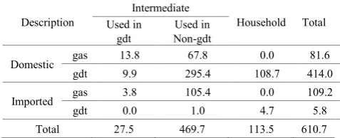
To determine the source of these issues consider now another aspect of the data on gas consumed in US as shown in Table A2. In this table the intermediate consumption of gas (sold either by “gas” or “gdt”) are divided into gas used by “gdt” and “non-gdt” sectors. This table shows that the “gdt” sector (as a gas using industry) is used 27.5 Mtoe gas. On the other hand this sector (i.e. “gdt”) sold 419.8 Mtoe of gas as a gas seller. Since “gdt” does not use resources to produce gas, this shows that transferred gas from “gas” sector to “gdt” sector is not included in the GTAP energy data in physical terms. Of course nothing is wrong here if we use this information to represent the net use of gas (as a source of energy) by sector. However, as it is evident from the GTAP regional I-O tables, if we use this data to measure the value of gas sold to the “gdt” sector in I-O tables, then the results will be misleading.

Table A2. US consumption of gas by major users in 2007 (Mtoe) Description Used in Intermediate Household Total

gdt Non-gdt Used in

Domestic gas 13.8 67.8 0.0 81.6 gdt 9.9 295.4 108.7 414.0 Imported gas 3.8 105.4 0.0 109.2 gdt 0.0 1.0 4.7 5.8 Total 27.5 469.7 113.5 610.7

According to the GTAP data base the value of gas sold to “gdt” in US (VDFM + VIFM) in 2007 is about $4.8 billion. This is about the value of net gas used in “gdt” as a source of energy (27.5 Mtoe reported in Table A2). This indicates that the US I-O table is missing the value of gas transferred from “gas” to “gdt” for distribution. The I-O tables of other regions suffer from the similar deficiency as well. Because of this deficiency, the cost share of gas in the cost structure of “gdt” is negligible in many regions in the GTAP data base as shown in Table A3. This deficiency undermines the linkages between the “gas”, “gdt”, and other sectors and badly affects the credibility of GTAP simulation results in response to the expansion in gas industry.

The GTAP data base version 8 misrepresents the monetary value of gas used by households also. As shown in tables A1 and A2, the GTAP data base shows that US households used about 113.5 Mtoe gas (gas plus gdt) in 2007. This is not very different for the corresponding figure reported by the DOE. However, the GTAP data base shows that US households purchased about $30 billion gas (domestic plus imported “gas” and “gdt”) in 2007, and this is very different from the corresponding reported value by DOE which is about $62 billion. This simple comparison shows that the GTAP data base badly underestimates values of gas used by households. Missing the value of gas transferred from “gas” to “gdt” causes this issue as well.

Table A3. Share of gas in the cost structure of “gdt” in GTAP data base version 8 by region

USA EU27 BRAZIL CAN JAPAN

4.4 5.8 53.1 1.5 1.1

CHIHKG INDIA C_C_Amer S_o_Amer E_Asia

15.2 0.3 27.8 13 10.4

Mala_Indo R_SE_Asia R_S_Asia Russia Oth_CEE_CIS

3.3 8.3 1.2 0.7 10.5

Oth_Europe MEAS_NAfr S_S_AFR Oceania

In addition to the above problems the split of gas between “gas” and “gdt” is counter intuitive. In general, the gas industry (including production and distribution) produces gas and sells it to major users such as power plants, major industries, commercial users, and households. In this process major users such as power plants and industries pay lower prices, and the commercial users and households pay a higher price. In general, the commercial and household users pay more because the distribution of gas through pipeline is costly. Now consider the implicit regional prices of gas sold by “gas” and “gdt” sectors, both obtained from the GTAP data base and presented in table A4. This table shows that the US implicit prices of gas sold by “gas” and “gdt” are about 304 $/toe and 269 $/toe with an average of 275 $/toe. According to the DOE data bases the US gas prices for household and power plants were about 507 $/toe and $283 $/toe, respectively, with an average of 359 $/toe in 2007. These figures show that the price of gas sold to households is much higher than the price of gas sold to power plants. But in

GTAP the price of gas sold by “gas” is much higher than the price of gas sold by “gdt”. In addition, these figures indicate that the GTAP implicit average price of gas is significantly below the actual average price of gas in US. Table A4 shows that the relationship between the gas prices sold by “gas” and “gdt” in some regions (e.g. EU and Canada) is consistent with what we expect to observe.

In conclusion, the above analyses indicate that:

 The GTAP data base ignores the link between “gas” and “gdt” and does not capture the values of gas sold from “gas” to “gdt” for distribution,

 The GTAP data base underestimates gas values used by commercial firms and households,

 The “gas” and “gdt” sectors in GTAP do not properly represent the production and distribution of gas as they operate in world.

Since these issues could affect the GTAP simulation results we modify the GTAP data base as outlined in the next sections.

Table A4. Implicit prices of gas sold by “gas” and “gdt” (values are in $/toe)

Region implicit price of gas sold by “gas” implicit price of gas sold by “gdt” Average implicit price of gas

USA 304.1 269.1 274.9

EU27 623.2 303.9 371.3

BRAZIL 169.7 172.5 170.7

CAN 509.2 216.1 468.4

JAPAN 310.3 310.3 310.3 CHIHKG 98.9 115.1 106.7 INDIA 236.2 236.3 236.3 C_C_Amer 318.0 198.4 249.8 S_o_Amer 106.0 71.2 90.4

E_Asia 123.7 416.8 237.9 Mala_Indo 685.5 222.6 419.3 R_SE_Asia 877.7 301.5 403.1 R_S_Asia 289.1 286.7 287.4 Russia 147.5 260.6 180.9 Oth_CEE_CIS 487.4 303.9 395.0 Oth_Europe 1475.7 396.1 1446.1 MEAS_NAfr 335.9 150.7 266.9

Corrections in gas and gdt sectors

Step 1: In this step we pooled the “gas” and “gdt” together and created a new sector which covers both production and

distribution of gas. In addition, regions are aggregated to 19 categories following the GTAP-BIO model aggregation scheme. The FlexAgg program is used in this step.

Step 2: Then we made the following adjustment in the data base with the pooled gas and gdt activities:

a. The GTAP regional values of gas sold to commercial users (services) and households are corrected according and the available data. We used the GTAPAdjust program to introduce the corrected values in the data base and maintain its balances.

b. The modified gas sector is divided into two sectors of “Gas” and “Gas-D” so that the former sells gas to industries, and the latter sells gas to services and households. The Split.com program is used to accomplish this task.

c. The values of gas sold from “Gas” to Gas-D” in each region are estimated and included in the data base, again using

the GTAPAdjust program.

The regional market values of gas sold by “Gas-D” inflated by 65% to represent the price difference between the price of gas for industries and commercial firms and household. The GTAPAdjust is used several times to handle this modification and reconstruct the cost structures of the new “Gas” and “Gas-D” sectors.

Appendix B: Original and modified production functions

Table B1. A representative production function in original GTAP-E original model

Top nest 𝑌𝑌 = �∝𝑉𝑉𝑉𝑉𝑉𝑉𝑉𝑉

(𝜎𝜎1−1

𝜎𝜎1)_{+ 𝛼𝛼}

𝑁𝑁𝑉𝑉𝑁𝑁1𝑁𝑁𝑉𝑉𝑁𝑁1 (𝜎𝜎1−1

𝜎𝜎1)_{+ ⋯ + 𝛼𝛼}

𝑁𝑁𝑉𝑉𝑁𝑁𝑛𝑛𝑁𝑁𝑉𝑉𝑁𝑁𝑛𝑛 (𝜎𝜎1−1

𝜎𝜎1)_�

( 𝜎𝜎1

𝜎𝜎1−1)

Where: ∝𝑉𝑉𝑉𝑉+ 𝛼𝛼𝑁𝑁𝑉𝑉𝑁𝑁1+ ⋯ + 𝛼𝛼𝑁𝑁𝑉𝑉𝑁𝑁𝑛𝑛= 1 and 𝜎𝜎1= 𝜎𝜎𝑉𝑉𝐸𝐸𝐸𝐸𝐸𝐸𝐸𝐸

Value added and energy nest

𝑉𝑉𝑉𝑉 = �𝛼𝛼𝑅𝑅𝑅𝑅 (𝜎𝜎2−1

𝜎𝜎2)_{+ 𝛼𝛼}

𝐿𝐿𝐿𝐿 (𝜎𝜎2−1

𝜎𝜎2)_{+ 𝛼𝛼}

𝑀𝑀𝑀𝑀 (𝜎𝜎2−1

𝜎𝜎2)_{+ 𝛼𝛼}

𝐾𝐾𝑉𝑉𝐾𝐾𝑉𝑉 (𝜎𝜎2−1

𝜎𝜎2)_�

( 𝜎𝜎2

𝜎𝜎2−1)

Where: 𝛼𝛼𝑅𝑅+ 𝛼𝛼𝐿𝐿+ 𝛼𝛼𝑀𝑀+ 𝛼𝛼𝐾𝐾𝑉𝑉= 1 and 𝜎𝜎2= 𝜎𝜎𝑉𝑉𝐸𝐸𝐸𝐸𝐸𝐸𝑉𝑉𝐸𝐸

Capital and energy nest 𝐾𝐾𝑉𝑉 = �∝𝑉𝑉𝑉𝑉

(𝜎𝜎3−1

𝜎𝜎3)_{+ 𝛼𝛼}

𝐾𝐾𝐾𝐾 (𝜎𝜎3−1

𝜎𝜎3)_�

( 𝜎𝜎3

𝜎𝜎3−1)

Where: 𝛼𝛼𝑉𝑉+ 𝛼𝛼𝐾𝐾= 1 and 𝜎𝜎3= 𝜎𝜎𝑉𝑉𝐿𝐿𝐾𝐾𝑉𝑉

Energy nest 𝑉𝑉 = �∝𝑉𝑉𝐿𝐿𝑉𝑉𝐿𝐿

(𝜎𝜎4−1

𝜎𝜎4)_{+ 𝛼𝛼}

𝑁𝑁𝑉𝑉𝐿𝐿𝑁𝑁𝑉𝑉𝐿𝐿 (𝜎𝜎4−1

𝜎𝜎4)_�

( 𝜎𝜎4

𝜎𝜎4−1)

Where: 𝛼𝛼𝑉𝑉𝐿𝐿+ 𝛼𝛼𝑁𝑁𝑉𝑉𝐿𝐿= 1 and 𝜎𝜎4= 𝜎𝜎𝑉𝑉𝐿𝐿𝑉𝑉𝑁𝑁

Non-Electricity nest 𝑁𝑁𝑉𝑉𝐿𝐿 = �∝𝐶𝐶𝐶𝐶

(𝜎𝜎5−1

𝜎𝜎5)_{+ 𝛼𝛼}

𝑁𝑁𝐶𝐶𝑁𝑁𝐶𝐶 (𝜎𝜎5−1

𝜎𝜎5)_�

( 𝜎𝜎5

𝜎𝜎5−1)

Where: 𝛼𝛼𝐶𝐶+ 𝛼𝛼𝑁𝑁𝐶𝐶= 1 and 𝜎𝜎5= 𝜎𝜎𝑉𝑉𝐿𝐿𝑁𝑁𝑉𝑉𝐿𝐿

Non-Coal nest 𝑁𝑁𝐶𝐶 = �∝𝑂𝑂𝑂𝑂

(𝜎𝜎6−1

𝜎𝜎6)_{+ 𝛼𝛼}

𝐺𝐺𝐺𝐺 (𝜎𝜎6−1

𝜎𝜎6)_{+ 𝛼𝛼}

𝑃𝑃𝑃𝑃 (𝜎𝜎6−1

𝜎𝜎6)_�

( 𝜎𝜎6

𝜎𝜎6−1)

Where: 𝛼𝛼𝑂𝑂+ 𝛼𝛼𝐺𝐺+ 𝛼𝛼𝑃𝑃= 1 and 𝜎𝜎6= 𝜎𝜎𝑉𝑉𝐿𝐿𝑁𝑁𝐶𝐶𝑂𝑂𝐸𝐸𝐿𝐿

Definitions: The variables and parameters used in the above equations are: αi’s represent share parameters; σi’s show substitution elasticities;

variables O, G, P, C, and EL demonstrate energy inputs including crude oil, gas, petroleum products, coal, and electricity, respectively; variables R, L, M, K stand for primary inputs including resources, labor, land, and capital, respectively; NEIi’s presents non-energy intermediate inputs; and

Table B2. A representative production function in modified GTAP-E original model

Top nest 𝑌𝑌 = �∝𝑉𝑉𝑉𝑉𝑉𝑉𝑉𝑉

(𝜎𝜎1−1

𝜎𝜎1)_{+ 𝛼𝛼}

𝑁𝑁𝑉𝑉𝑁𝑁1𝑁𝑁𝑉𝑉𝑁𝑁1 (𝜎𝜎1−1

𝜎𝜎1)_{+ ⋯ + 𝛼𝛼}

𝑁𝑁𝑉𝑉𝑁𝑁𝑛𝑛𝑁𝑁𝑉𝑉𝑁𝑁𝑛𝑛 (𝜎𝜎1−1

𝜎𝜎1)_�

( 𝜎𝜎1

𝜎𝜎1−1)

Where: ∝𝑉𝑉𝑉𝑉+ 𝛼𝛼𝑁𝑁𝑉𝑉𝑁𝑁1+ ⋯ + 𝛼𝛼𝑁𝑁𝑉𝑉𝑁𝑁𝑛𝑛= 1 and 𝜎𝜎1= 𝜎𝜎𝑉𝑉𝐸𝐸𝐸𝐸𝐸𝐸𝐸𝐸

Value added and energy nest

𝑉𝑉𝑉𝑉 = �𝛼𝛼𝑅𝑅𝑅𝑅 (𝜎𝜎2−1

𝜎𝜎2)_{+ 𝛼𝛼}

𝐿𝐿𝐿𝐿 (𝜎𝜎2−1

𝜎𝜎2)_{+ 𝛼𝛼}

𝑀𝑀𝑀𝑀 (𝜎𝜎2−1

𝜎𝜎2)_{+ 𝛼𝛼}

𝐾𝐾𝑉𝑉𝐾𝐾𝑉𝑉 (𝜎𝜎2−1

𝜎𝜎2)_�

( 𝜎𝜎2

𝜎𝜎2−1)

Where: 𝛼𝛼𝑅𝑅+ 𝛼𝛼𝐿𝐿+ 𝛼𝛼𝑀𝑀+ 𝛼𝛼𝐾𝐾𝑉𝑉= 1 and 𝜎𝜎2= 𝜎𝜎𝑉𝑉𝐸𝐸𝐸𝐸𝐸𝐸𝑉𝑉𝐸𝐸

Capital and energy nest 𝐾𝐾𝑉𝑉 = �∝𝑉𝑉𝑉𝑉

(𝜎𝜎3−1

𝜎𝜎3)_{+ 𝛼𝛼}

𝐾𝐾𝐾𝐾 (𝜎𝜎3−1

𝜎𝜎3)_�

( 𝜎𝜎3

𝜎𝜎3−1)

Where: 𝛼𝛼𝑉𝑉+ 𝛼𝛼𝐾𝐾= 1 and 𝜎𝜎3= 𝜎𝜎𝑉𝑉𝐿𝐿𝐾𝐾𝑉𝑉

Energy nest 𝑉𝑉 = �∝𝑉𝑉𝐿𝐿𝑉𝑉𝐿𝐿

(𝜎𝜎4−1

𝜎𝜎4)_{+ 𝛼𝛼}

𝑁𝑁𝑉𝑉𝐿𝐿𝑁𝑁𝑉𝑉𝐿𝐿 (𝜎𝜎4−1

𝜎𝜎4)_�

( 𝜎𝜎4

𝜎𝜎4−1)

Where: 𝛼𝛼𝑉𝑉𝐿𝐿+ 𝛼𝛼𝑁𝑁𝑉𝑉𝐿𝐿= 1 and 𝜎𝜎4= 𝜎𝜎𝑉𝑉𝐿𝐿𝑉𝑉𝑁𝑁

Coal-Gas and Oil-Petroleum nest

𝑁𝑁𝑉𝑉𝐿𝐿 = �∝𝐶𝐶𝐺𝐺𝐶𝐶𝐺𝐺 (𝜎𝜎5−1

𝜎𝜎5)_{+ 𝛼𝛼}

𝑂𝑂𝑃𝑃𝑂𝑂𝑃𝑃 (𝜎𝜎5−1

𝜎𝜎5)_�

( 𝜎𝜎5

𝜎𝜎5−1)

Where: 𝛼𝛼𝐶𝐶𝐺𝐺+ 𝛼𝛼𝑂𝑂𝑃𝑃= 1 and 𝜎𝜎5= 𝜎𝜎𝑉𝑉𝐿𝐿𝐶𝐶𝐺𝐺𝑂𝑂𝑃𝑃

Coal and gas nest 𝐶𝐶𝐺𝐺 = �∝𝐶𝐶𝐶𝐶

(𝜎𝜎6−1

𝜎𝜎6)_{+ 𝛼𝛼}

𝐺𝐺𝐺𝐺 (𝜎𝜎6−1

𝜎𝜎6)_�

( 𝜎𝜎6

𝜎𝜎6−1)

Where: 𝛼𝛼𝐶𝐶+ 𝛼𝛼𝐺𝐺= 1 and 𝜎𝜎6= 𝜎𝜎𝑉𝑉𝐿𝐿𝐶𝐶𝐺𝐺

Definitions: The variables and parameters used in the above equations are: αi’s represent share parameters; σi’s show substitution elasticities;

variables G, C, OP and EL demonstrate energy inputs including gas, coal, oil and petroleum products, and electricity, respectively; variables R, L, M, K stand for primary inputs including resources, labor, land, and capital, respectively; NEIi’s presents non-energy intermediate inputs; and finally Y is

the final output.

REFERENCES

[1] Advanced Resources International. EIA/ARI World shale sas and shale oil resource assessment, Advanced Resources International Inc. Arlington, VA, USA, 2013.

[2] U.S. Department of Energy. Annual energy outlook. Washington DC, USA, 2013.

[3] S. Brown, S. Gabriel, R. Egging. Abundant shale gas resources: Some implications of energy policy, Resources for the Future. USA, 2010.

[4] S. Paltsev, D. Jacoby, J. Reilly, Q. Ejaz, F. O'Sullivan, J. Morris, S. Rausch, N. Winchester, O. Kragha. The future of U.S. natural gas production, use, and trade, Energy Journal, 39: 5309-5321. 2011.

[5] D. Jacoby, F. O'Sullivan, S. Paltsive. The influence of shale gas on U.S. energy and environmental policy, MIT Joint Program on the Science and Policy of Global Change, USA, 2012.

[6] IHS Global Insight. The economic and employment contributions of shale gas in the United States, IHS Global Insights (USA) Inc., Washington DC, USA, 2011.

[7] Citi GPS. Energy 2020: North America, the new Middle East?

Citi GPS: Global Perspecitves and Solutions, 2012.

[8] V. Arora. Aggregate impacts of recent U.S. ratural gas trends.

U.S. Department of Energy, Washington DC, USA, 2013 [9] K. Sarica, W. Tyner. Alternative policy impacts on US GHG

emissions and energy security: A hybrid modeling approach, Energy Economics, 40:40-50, 2013.

[10]F. Taheripour, W. Tyner, K. Sarica. Shale gas boom, trade and environmental policies: Global economic and environmental analyses in a multidisciplinary modeling framework, In R.E. Hester, and R. Harrison eds. Issues in Environmental Science and Technology, Vol. 39 Fracking, Cambridge, UK, Royal Society of Chemistry, 2014.

[11]T. Hertel. Global trade analysis, modeling and applications, Cambridge University Press, Cambridge, UK, 1997. [12]J.Burniaux, T. Truong. GTAP-E: An energy-environmental

version of the GTAP model,GTAP technical paper No. 16, Center for Global Trade Analysis, Purdue University, West Lafayette, IN, USA, 2002.

[13]R. McDougall, A. Golub. GTAP-E release 6: A revised energy-environmental version of the GTAP model, GTAP Technical Paper No. 15, Center for Global Trade Analysis, Purdue University, West Lafayette, IN, USA, 2007. [14]F. Taheripour, D. Birur, T. Hertel, W. Tyner. Introducing

USA, 2007.

[15]T. Hertel, A. Golub, A. Jones, M. O'hare, R. Plevin, D. Kammen. Effects of US maize ethanol on global land use and greenhouse gas emissions: Estimating market-mediated responses, Bioscience 60(3), 223-231, 2010.

[16]Energy Information Administration. Emissions of greenhouse gases in the United States 2009, U.S. Department of Energy, Washington, DC, USA, 2011.

[17]B. Narayanan, A. Aguiar, R. McDougall. Global Trade, Assistance, and Production: The GTAP 8 Data Base, Center for Global Trade Analysis, Purdue University, West Lafayette, IN, USA, 2012.