Estimation of the volatility function: Non parametric and semiparametric approaches

L on d on S ch o o l o f E con om ics and P o litic a l S cien ce

Department of Statistics

E stim a tio n o f th e V ola tility Function:

N on -p aram etric and Sem iparam etric A pproaches

Panagiotis A vram idis

M a y 2004

T hesis s u b m itte d to th e U n iversity o f London in p a rtia l fulfillm ent

UMI Number: U 195150

All rights reserved

INFORMATION TO ALL U SE R S

The quality of this reproduction is d ep en d en t upon the quality of the copy subm itted.

In the unlikely even t that the author did not sen d a com plete m anuscript

and there are m issing p a g e s, th e se will be noted. Also, if material had to be rem oved, a note will indicate the deletion.

Dissertation Publishing

UMI U 195150

Published by ProQ uest LLC 2014. Copyright in the Dissertation held by the Author. Microform Edition © ProQ uest LLC.

All rights reserved. This work is protected against unauthorized copying under Title 17, United S ta tes C ode.

ProQ uest LLC

I

K £ S £ S

A b s tra c t

We investigate two problems in modelling tim e series d a ta th a t exhibit conditional

heteroscedasticity. The first p art deals with the local m axim um likelihood estim ation

of volatility functions which are in the form of conditional variance functions. The

existing estim ation procedures yield plausible results. Yet, they often fail to take

into account special features of the d ata at th e cost of reduced accuracy of predic­

tion. More precisely, m any of the param etric and nonparam etric conditional variance

models ignore the fact th a t the error distribution departs significantly from gaussian

distribution. We propose a novel nonparam etric estim ation procedure th a t replaces

popular local least squares m ethod with local m axim um likelihood estim ation. In­

tuitively, using inform ation from the error distribution improves the estim ators and

therefore increases th e accuracy in prediction. This conclusion is proved theoreti­

cally and illustrated by numerical examples. In addition, we show th a t the proposed

estim ator adapts asym ptotically to the error distribution as well as to the mean re­

gression function. A pplications w ith real d a ta examples d em onstrate the potential

use of the adaptive maxim um likelihood estim ator in financial risk m anagem ent.

T he second p art deals with the variable selection for a particular class of semipara-

metric models known as the partial linear models. T he existing selection m ethods are

com putationally dem anding. The proposed selection procedure is com putationally

more efficient. In particular, if P and Q are the num ber of linear and nonparam etric

candidate regressors, respectively, then the proposed procedure reduces the order of

the num ber of variable subsets to be investigated from 2Q+P to 2Q + 2P. At the same

time, it m aintains all the good properties of existing m ethods, such as consistency.

The la tter is proven theoretically and confirmed num erically by sim ulated examples.

The results are presented for the mean regression function while the generalization

A c k n o w le d g e m e n t

I am deeply grateful to my supervisor Professor Qiwei Yao for being a limitless

source of knowledge and for all his inspiration. I would like to th a n k my MSc tu to r Dr

Jerem y Penzer for helping me build the necessary foundations and all the people from

the D ep artm en t of S tatistics for their ongoing sup port. T he financial sponsorship from

ESRC is gratefully acknowledged. Moreover, I w ant to th a n k my physics professor

Mr D im itris G iannakos for his encouragem ent from th e early stages of my studies.

F urtherm ore, I would like to th a n k my office m ates whose presence m ade this

process a joyful and enriching journey. Special th an k s to Jaya, Yorghos and Diego

w ith whom I sta rte d this journey and who paved its way. I am also very grateful to

all my friends here in London and those back home, for sharing w ith me th e good

and th e bad m om ents during these years and giving m e th e courage to succeed.

Finally, I would like to th an k my uncle Iakovos, an d my b ro th er Y iannis, for their

unconditional love and support. Last here b u t first in my h eart, two people who

have defined my life so far: my father for being a stim ulatin g source of wisdom and

To m y parents, K onstantinos and Eirini,

m y greatest teachers of life,

fo r their endless love.

In loving m em ory o f m y grandmother,

II poaQscnq

A v e v r v x ijs 9 dvcrrvxiJS sCpau dev £ ^ e r a ( u .

IIX pv e v a 'Kpd'ypa p£ x&P&v gtov i/ov p o v TTOivra

fiaC,u-7TOV GTT}V (jL^aXr) 7rpOG0£GL (rr)U TTpOG0£Gl TLJIS 7T0V piGLj)

7TOV £X£L TOGOVq OLpL0pOVq, 8cU £ipOLl £7LJ £K£l

air' T£s iroXXiq povdbeq pea. M eq g t' oXlko ttogo

dev api0pr]0pna. K l a v r fj tj x a P& P' OipneL.

Kujvgtolvtlvoc; 77. Kafionpigq (1897)

Addition

I do not question whether I am happy or unhappy.

Yet there is one thing that I keep gladly in m ind

-that in the great addition (their addition -that I abhor)

that has so m any numbers, I am not one

of the m any units there. In the final sum

I have not been calculated. A n d this jo y suffices me.

C on ten ts

1 I n t r o d u c t i o n in v o la til ity m o d e llin g 12

2 L o c a l L in e a r M a x im u m L ik e lih o o d E s t i m a t o r 19

2.1 M odel and conditional likelihood function ... 19

2.2 Local polynom ial f i t t i n g ... 20

2.3 T he local linear m axim um likelihood e s tim a to r ... 2 1 2.4 A sym ptotic properties of th e M L -e stim a to r... 24

2.4.1 C o n s is te n c y ... 26

2.4.2 A sym ptotic norm ality ... 28

2.5 Im plem entation and bandw idth s e le c tio n ... 40

2.6 C om parison of M LE w ith existing e s tim a to rs ... 42

2.7 Sim ultaneous estim ation of the m ean and variance f u n c tio n ... 46

2.7.1 C onsistency of th e joint e s ti m a t o r ... 49

2.7.2 A sym ptotic norm ality of th e joint e s t i m a t o r ... 53

2.8 N um erical a p p lic a tio n s ... 6 6 2.8.1 N um erical exam ple 2 . 1 ... 67

2.8.2 N um erical exam ple 2 . 2 ... 70

3 A d a p ti v e M a x im u m L ik e lih o o d E s t i m a t o r 72 3.1 M otivation and prelim inary r e s u l t s ... 72

3.2.1 A sym ptotic properties of the ad aptive M L -estim ator ... 82

3.3 N um erical a p p lic a tio n s ... 92

3.3.1 N um erical exam ple 3 . 1 ... 92

3.3.2 N um erical exam ple 3 . 2 ... 98

4 A T w o - S te p C r o s s - V a lid a tio n S e le c tio n M e t h o d F o r P a r t i a l l y L in e a r M o d e ls 100 4.1 Existence of a p artially linear regression m o d e l... 100

4.2 Selection of th e nonparam etric c o m p o n e n t ... 103

4.3 Selection of param etric com ponent ... 113

4.4 B and w id th selection ... 120

4.5 Extension to th e variance fu n c tio n ... 121

4.6 N um erical e x a m p le s ... 122

4.6.1 M ean regressors s e le c tio n ... 1 2 2 4.6.2 M ean regressors selection w ith two p r o c e s s e s ... 124

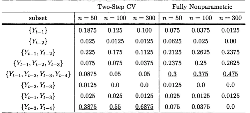
4.6.3 V ariance regressors s e le c tio n ... 126

5 A p p lic a tio n s o f t h e a d a p t iv e M L - e s ti m a to r t o V a lu e a t R is k 128 5.1 In tro d u ctio n to VaR theory ... 128

5.2 R eal d a ta a p p l i c a t i o n s ... 130

5.2 .1 Stock indices ... 131

5.2.2 S t o c k s ... 147

5.2.3 Exchange r a t e s ... 155

5.3 C o n c lu sio n ... 159

List o f Tables

2.1 Efficiency for ^-distribution w ith k degrees of f r e e d o m ... 45

3.1 B andw idth for error density and derivative estim a to r... 95

4.1 P robabilities of nonparam etric regressors selection: th e leave-one-out

C V ... 123

4.2 P robabilities of selection based on the M CCV w ith Yt-3, Yt - 4 th e non­

p aram etric regressors... 123

4.3 P robabilities of nonparam etric regressors selection: th e leave-one-out

C V ... 125

4.4 P robabilities of selection based on th e M CCV w ith X t th e nonp ara­ m etric regressor... 125

4.5 P robabilities of th e nonparam etric regressors: the leave-one-out CV . 127

4.6 P robabilities of selection based on the M CCV w ith Yt-2 for non para­

m etric r e g r e s s o r ... 127

5.1 Stock indices: deviation measures and hypothesis te s ts ... 142

5.2 Stock indices: ratio of exceeding observations ( x lO -2 ) for a=5% . . . 145

5.3 Stock indices: ratio of exceeding observations ( x lO -2 ) for a = l% . . . 146

5.4 Stocks: n onp aram etric Cross-Validation function ( x lO -6 ) ... 148

5.5 Stocks: M ean A bsolute D eviation E rror ( x lO -4 ) and square-R

5.6 Stocks: exceedence ratio (x lO -2 ) for a = 5%... 150

5.7 Exchange rates: deviation m easures and hypothesis te s ts ... 157

List o f F igures

2.1 P lo t of sta n d a rd deviation function a ( x1,0:2): (a) T he tru e function

(b) th e M L -estim ator for gaussian errors... 6 8

2.2 (i) P lo t of AM ISE vs bandw idth h using (a) th e tru e value of cr(.) and

its derivatives (b) th e M L-estim ates. (ii) B ox-Plot of M AD E for the

LSE and M LE for gaussian and ^ -d is trib u te d errors w ith k = 6 and

k = 14 d .f... 69

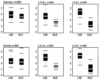
2.3 Box-Plot of th e M ADE for the LSE and M LE for gaussian and

tk-d istrib u tetk-d error w ith k = 2 and A; = 15 d.f. and n = 200, 500... 71

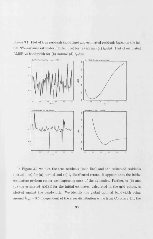
3.1 P lo t of tru e residuals (solid line) and estim ated residuals based on th e

initial N W -variance estim ates (d otted line) for (a) norm al-(c) t3-dist.

P lo t of estim ated AM SE vs b andw idth for (b) norm al (d) t3-dist. . . 93

3.2 D ensity estim ators based on the estim ated errors et for (a) gaussian

and (b) t3 error d istrib u tio n ... 94

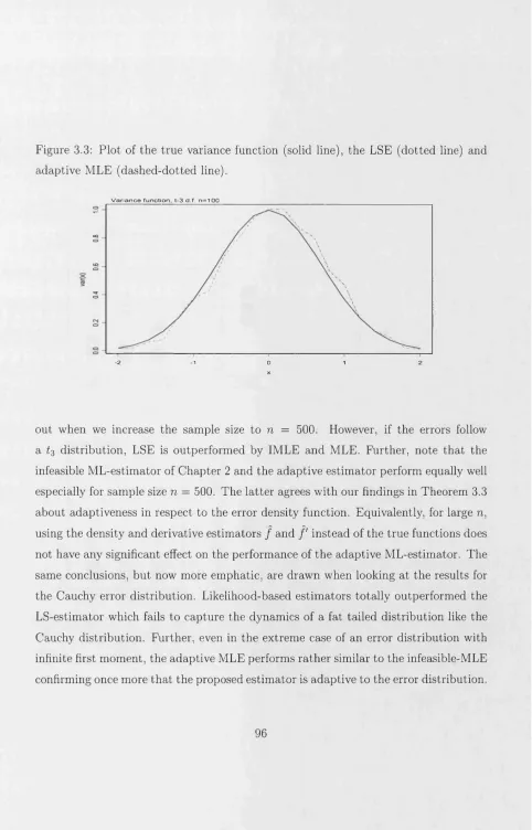
3.3 P lo t of the tru e variance function (solid line), th e LSE (d otted line)

and ad aptive M LE (dashed-dotted line)... 96

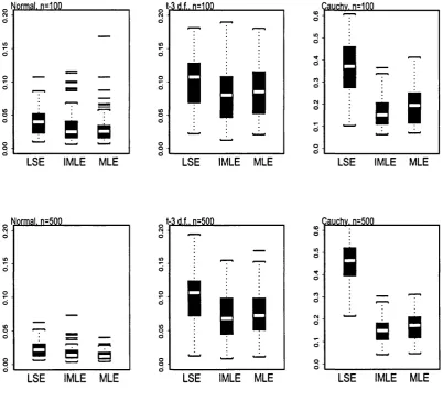
3.4 B ox-Plot of th e M A D E of th e LSE, th e Infeasible-M LE and th e adap­

tive M LE for gaussian, 13 and Cauchy errors for n = 100, 500... 97

3.5 B ox-Plot of th e M AD E of the LSE, th e Infeasible-M LE and th e adap­

tive M LE for gaussian, t§ and £14 d istrib u ted errors w ith n = 100, 500. 99

5.2 R eturns and squared retu rn s autocorrelation fun ctio n... 133

5.3 SP R eturns: Series and conditional sta n d a rd deviation, LSE and MLE. 135

5.4 D J R eturns: Series and conditional stan d ard deviation, GARCH and

E G A R C H ... 136

5.5 F T S E R eturns: Series and conditional sta n d a rd deviation, EGARCH

and M L E ... 137

5.6 DAX R eturns: Series and conditional stan d ard deviation, G ARCH and

L S E ... 138

5.7 N orm al probability plot for th e SP500 and DAX re tu rn s ... 139

5.8 N orm al probability plot for SP500 and D J residuals from G ARCH model. 140

5.9 M ean log-Likelihood vs percentile for GARCH (solid), G A RCH-2 (small

dashed), M LE (large dashed), LSE (d o tte d )... 151

5.10 Realized an d predicted volatility for INL an d JP M : LSE (solid top),

G ARCH (dashed top), M LE (solid bo ttom ), G A RCH-2 (dashed bo ttom ). 153

5.11 M ean log-Likelihood using 2-dist. vs percentile for th e stock average:

LSE (dotted ), G ARCH (solid), MLE (large dashed), G A RCH-2 (small

d ash ed )... 154

5.12 Realized and predicted volatility for exchange rates, G A RCH (dashed-

C hapter 1

In trod u ction in v o la tility m od ellin g

T here is a wide range of tim e series d a ta sets where th e sam ple variation changes

over tim e, a phenom enon known as heteroscedasticity. For exam ple, in financial m ar­

kets, large m ovem ents tend to be followed by large m ovem ents and th e same p a tte rn

applies for th e sm all movements. T he fluctuating behavior of th e finance m arket is

referred to as the “volatility” . V olatility is typically characterized by th e conditional

variance or sta n d a rd deviation. Given th e extended num ber of applications, m od­

elling, estim ating and predicting th e volatility, in th e form of conditional variance,

have a ttra c te d much of th e atten tio n in th e recent research work. As a result, a large

num ber of volatility models and estim ation m ethods have been developed.

U ndoubtedly, using conditional argum ents, th e m ost im p o rta n t param etric models

are th e A uto-Regressive C onditional H eteroscedastic (ARCH) m odel (Engle 1982)

and th e G eneralized A uto-Regressive C onditional H eteroscedastic (GARCH) model

(Bollerslev 1986). Due to th e practicality and relatively good perform ance, GARCH

rem ains one of th e m ost frequently employed conditional variance models in finance.

In consequence of its success, variations of GARCH app eared in literatu re including

the p opular exponential-G A R C H (Nelson 1991) and th e G A RCH -in-M ean (Engle,

Lilien, and R obins 1987). See also G ourieroux (1997), H am ilton (1994) and Bollerslev,

Various non-param etric procedures for estim ating conditional variance functions,

have been proposed. H ardle and Tsybakov (1997) introduce a kernel estim ator based

on the decom position a 2(x) = E ( Y 2\ X = x) — ( E ( Y \ X = x ) ) 2. However, th e proposed

estim ator m ay n ot be positive and it also creates large bias. R u p p ert, W and, Holst,

and Hossjer (1997) for i.i.d. and Fan and Yao (1998) for tim e series, stu d y a residual-

based estim ato r in conjunction w ith local kernel sm oothing. T h e resulting estim ator

is m ean regression ad ap tiv e1. Likewise, M uller and S tadtm iiller (1987) obtain th e

uniform convergence rates for an alternative m ean regression adaptive estim ator, th e

kernel-sm oothed local variance estim ator.

In addition, m any of the models introduced in th e m ore general settin g of mean

regression function can be im plem ented for conditional variance function after some

m odification. Recall the well-known N adaraya-W atson estim ato r (N adaraya 1964 and

W atson 1964) and th e bou nd ary Gasser-M iiller kernel regression estim ator (Gasser

and M uller 1984). However, b o th estim ators suffer from draw backs. Particularly,

the N adaraya-W atson estim ato r results in an increase in th e bias while Gasser-M iiller

estim ator yields large asym ptotic variance. On the o th er hand, the com bination of

local polynom ial approxim ation and least squares estim ation leads to th e local poly­

nom ial kernel estim ato r (Stone 1977 and m ore recently, Fan 1992, R u p p ert and W and

1994). T he local polynom ial kernel estim ator ad ap ts auto m atically to estim ation at

th e boundaries. Equivalently, it does not suffer from th e lack of sufficient observa­

tions a t th e boundaries, a phenom enon known as “boundary effects”. Moreover, Fan

(1993) showed th a t it achieves th e highest “linear m in im a x efficiency” , in the sense of

m inim um possible suprem um of A sym ptotic M ean Square E rror, am ong th e class of

linear sm oothers. A detailed picture ab out th e p roperties an d advantages of th e local

polynom ial sm oother can be found in W and and Jones (1995) and Fan and Gijbels

(1996). See also Fan and Yao (2003) for an overview of th e non param etric estim ation

m ethods including th e local polynom ial estim ator.

An alternativ e approach to least squares m ethod is th e m axim um likelihood estim a­

tion. O ur m otivation stem s from th e param etric theory and particu larly from the fact

th a t m axim um likelihood estim ator achieves asym ptotically th e C ram er Rao bound

of th e variance of th e unbiased estim ators. It is un d ersto o d th a t using inform ation

on the error d istrib u tio n improves the perform ance of th e estim ato r and increases the

accuracy of th e prediction. A lthough not very frequently employed, likelihood func­

tion in nonp aram etric framework is not to tally unknown. Simonoff (1996) and H jort

and Jones (1996) use local likelihood in th e context of density function estim ation

while Stanisw alis (1989) derives th e asym ptotic properties of a kernel likelihood-based

estim ator of a regression function for th e case of i.i.d. d ata. F urther, Linton and Xiao

(2 0 0 1) propose a local polynom ial, likelihood-based, estim ato r of th e m ean function

th a t ad ap ts to th e error distribution. B andw idth selection an d confidence intervals

are discussed by Fan, Farm en, and Gijbels (1998). O n th e o th er hand, little appears

in the literatu re on th e use of likelihood estim ation for th e volatility function. Yu and

Jones (2004) introduce a m axim um likelihood estim ato r for th e variance com ponent.

However, their approach is a pseudo-likelihood estim ation since they use gaussian

distribu tio n in stead of th e unknow n error distribution.

We propose a novel, general approach to th e use of th e likelihood function in the

estim ation of the conditional variance function. In C h ap ter 2 we assum e th a t the

error d istrib u tio n is known and we introduce th e local linear M axim um Likelihood

estim ator of th e conditional variance function. Specifically, th e estim ator is a lo­

cal linear approxim ation of th e log-standard deviation function com bined w ith the

likelihood function as th e minimizing estim ation function. T he introduction of the

log-transform ation in th e local polynom ial fitting is also pivotal. T he estim ator of

the variance function should be positive, a p rop erty im plied by th e log-transform ation

w ith no need for fu rth er restrictions. However, th e asy m ptotic results of th e estim a­

to r suggest th a t th e effect of th e log-transform ation on th e squared bias depends on

any gain in asym ptotic variance may be overshadowed by an increase of the squared

bias, see Yu and Jones (2004) for a sim ilar conclusion. In an a tte m p t to quantify the

gain due to the use of likelihood function, we perform a direct theoretical com parison

based on the A sym ptotic M ean Square Error, between th e likelihood estim ator and

existing estim ators. T he com parison applies for large n as it involves th e asym ptotic

properties of the estim ators. T he results reflect th e in itial im pression th a t use of the

inform ation from th e error distribution improves th e perform ance of th e estim ator

especially when there is significant dep artu re from th e assum ption of gaussian errors.

A lthough th e n on param etric conditional heteroscedastic m odel includes directly

the conditional m ean function, th e above results were derived assum ing it is known.

In order to extend these results for the more realistic case of unknow n m ean func­

tion, we continue in C h ap ter 2 w ith th e investigation of a jo in t m axim um likelihood

estim ator for b o th th e m ean and variance function. By establishing th e asym ptotic

properties of th e jo in t estim ator, we identify sufficient conditions for th e adaptive­

ness of th e variance function estim ator w ith respect to th e m ean function estim ator.

T he term “adaptiveness” refers to th e characteristic th a t w ith ou t knowing th e mean

function m (.), we can estim ate th e variance function asym ptotically as well as if m (.)

was known. Equivalently, adaptiveness implies th a t th e use of th e estim ated mean

function instead of th e tru e m ean function has no effect on th e first order asym ptotic

properties of th e variance estim ator. T he identified condition for adaptiveness is the

sym m etry of th e error distribution. It is a well known requirem ent for sim ilar conclu­

sion ab o u t location and scale param eters w ithin th e context of param etric regression,

see Severini (2000). Furtherm ore, at th e end of C h ap ter 2, we present two num erical

exam ples th a t reinforce th e conclusions draw n from th e direct theoretical comparison.

T here is no d o u b t th a t the condition of known error d istrib u tio n is fairly restric­

tive. For this reason th e estim ator from C h ap ter 2 is referred to as th e infeasible-

M axim um Likelihood estim ator. It is therefore u n d erstoo d th a t th is condition needs

In C h apter 3, we propose a new, likelihood-based estim ato r th a t requires no prior

knowledge of th e error distribution. More precisely, we replace th e error density and

its derivatives by th e nonparam etric kernel estim ators to o btain an estim ate for the

score function (the first derivative of th e likelihood function) and th e Hessian m atrix

(the second derivative of th e likelihood function). T hen, th e new estim ator is the one

step Newton R aphson likelihood estim ator calculated using th e estim ated score func­

tion and H essian m atrix. It is proven th a t it shares th e sam e asym ptotic properties

w ith the infeasible M axim um Likelihood estim ator. T he la tte r implies adaptiveness

w ith respect to th e error distribution. Hence, we call this estim ator the adaptive

M axim um Likelihood estim ator. Note th a t by requiring no p articu la r form for the

error density, th e results apply for any density function / ( . ) th a t satisfies the im­

posed regularity conditions. This makes th e estim ato r m ore flexible especially when

the error d istrib u tio n d ep arts significantly from gaussian distrib ution. C h apter 3 con­

cludes w ith sim ulated exam ples in order to evaluate num erically the perform ance of

the adaptive estim ato r in com parison w ith th e infeasible estim ato r as well as other

estim ators e.g. th e Least Squares estim ator.

A nother im p o rtan t issue in modelling conditional variance function is the choice of

the variables used as regressors in the model. T he non param etric m odel introduced

in C h ap ter 2 assum ed a fixed, d-dimensional, set of variables. However, there is

little probability th a t th is set of variables is known a priori. M ore often, we have

a restricted num ber of can didate variables w ith some of th em having no significant

effect on th e dependent variable. In th a t case, we need to include only th e significant

predictors. T h e reason is th a t th e convergence ra te and consequently th e perform ance

of th e non param etric estim ator decreases as th e num ber of regressors increases, a

phenom enon known as “the curse of dimensionality” . I t is therefore critical th a t the

included regressors have significant effect on th e d ependent variable. T he selection

of th e regressors is usually based on th e m inim ization of a loss function, th e choice

nonparam etric context include, am ong others, th e C ross-V alidation criterion (Cheng

and Tong 1992, 1993) and the equivalent of th e F in al P rediction E rror criterion

(T jpstheim and A uestad 1994). Yao and Tong (1994) establish asy m p to tic results for

the Cross-V alidation criterion based on kernel estim ation. T h eir approach includes

tim e series. Correspondingly, the developm ents in variable selection in linear models

have been sub stan tial. T he Akaike inform ation criterion (Akaike 1974, S hibata 1981),

th e C ross-V alidation (Stone 1974, Shao 1993) and th e G eneralized-Cross V alidation

criterion (Craven and W ahba 1979) are the m ost frequently used m odel selection

procedures. See also Wei (1992) for an overview on th e problem of variables selection

for linear models. Here, in parallel to the issue of variables selection, we focus on

the form of th e conditional variance function. It is well known th a t nonparam etric

estim ators converge more slowly th a n param etric estim ators, see Robinson (1988)

and Fan (1993). T his m eans th a t if th e tru e m odel contains a linear com ponent then

nonparam etric estim ators will not be as efficient as p aram etric estim ators. In th a t

case a m ore flexible m odel form needs to be introduced. T his new class of models is

sem iparam etric and is known as partially linear models.

Consequently, in C h ap ter 4, we deal w ith th e problem of th e variable selection

for the sem iparam etric class of partially linear regression models. Following an idea

introduced by G ao and Tong (2002), we propose a novel, co m pu tation ally efficient,

variable selection procedure for th e class of p artially linear models. Particularly, a two

step selection procedure is proposed. At the first step, we select th e nonparam etric

regressors based on a Cross-V alidation criterion applied to th e residuals from linear

regression w ith all th e candidate regressors. T hen, given th e selected nonparam etric

variables, we use a param etric Cross-Validation criterion to remove any unnecessary

linear regressors. It is proven th a t the proposed selection procedure is consistent. T he

innovation here is th a t when calculating the residuals a t th e first step we include all th e

linear regressors (even those th a t are proven insignificant a t th e second step) and then

th a t should be considered which effectively leads to a significant reduction in the

com putations. We should m ention here th a t, though presented for a m ean regression

model, th e generalization of th e proposed selection m eth od to th e variance function

is straightforw ard an d is discussed in a separate section. Sim ulation examples are

presented a t the end of C h ap ter 4 to illustrate num erically th e consistency as well as

the reduction in the com putations.

In finance, volatility is often linked to th e concept of risk. W ith in the risk theory,

one of the m ost frequently employed m easures is th e “ Value at R i s k” (VaR). Hence,

in C hapter 5, we im plem ent th e proposed nonparam etric m eth od for estim ating con­

ditional heteroscedastic models in connection w ith the prediction of the VaR. Using

real d ata, we calculate th e VaR along w ith other perform ance te sts and deviation

measures in order to com pare the adaptive M L-estim ator w ith existing param etric

and nonparam etric estim ators. We use th ree different types of financial d a ta sets

i.e. stock-indices, stocks and exchange rates. T hey were chosen on th e grounds th a t

financial d a ta sets often exhibit heteroscedasticity while a t th e sam e tim e are heavy

tailed. T he la tte r is im p o rtan t because as we shall see in th e following chapters the

im provem ent a ttrib u te d to th e proposed estim ator becomes m ore ap p aren t when ana­

lyzing heavy tailed d a ta sets. C h ap ter 5 ends w ith a sum m ary of th e m ain conclusions

C hapter 2

Local Linear M axim um L ikelihood

E stim ator

2.1

M od el and conditional lik elih ood fu n ction

T he m odel th a t we are going to stu d y is a non-param etric regression conditional

heteroscedastic model. Let {Y^X*} be a strictly statio n ary process w ith scalar Yt

and d-dim ensional X.J = ( X ^ i,. . . , X tyd)- D enote by m : Md —> R th e conditional

m ean function, m (x ) = E(Yrf|X f = x), and a 2 : R d —► M+ th e conditional variance

function cr2(x) = V a r ^ X * = x) > 0. Define

- -

<2 I»

It is easy to see th a t E(ef|X f) = 0 and Var(e*|X*) = 1. A ssum e th a t et are i.i.d. and

call / ( . ) th e error density function. A t this stage, we assum e th a t th e error density

is known. We are in terested in estim ating the variance function and we are going to

do this for b o th cases of known and unknown m ean function. From (2.1) we get

w ith X t,i = Yt-i for i = 1, . . . ,d, then model (2.2) is an autoregressive conditional

heteroskedastic non-linear tim e series model. Hence, we will n o t assume indepen­

dence between Yt and X t , though we will impose some m ixing conditions necessary

for th e derivation of th e asym ptotic properties. Using equation (2.1) we have th a t

th e conditional density function of Yt |X f and th e error density are related through

/ r |x ( ! / | x ( = x ) = / ( ^ f M ) * \ a ( x ) / <t(x)

Consequently, the conditional log-likelihood function is defined

U Y |X ) = f > g f ( Yt ~ - X > g < r ( X , ) (2.3)

t- i l A

where Y = ( Y ,,. .. ,Y „)T, X = ( X j \ . .. ,X £ ).

2.2

Local p olyn om ial fittin g

T he local polynom ial fitting is a useful tool for th e estim ation of unknow n functions.

W and and Jones (1995), Fan and Gijbels (1996), am ong others, establish th e asym p­

totic properties of local polynom ial estim ators for th e m ean regression function. T he

m ain idea is th a t we tre a t the unknown function as a polynom ial in a small neighbor­

hood and by estim ating th e coefficients of th is polynom ial we o b tain an approxim ation

of th e function. T he choice of th e order of th e approxim ation has an effect on th e esti­

m ator. As Fan and G ijbels (1996) point out, “odd order polynomials are preferable to

even order polynomials fits” a conclusion draw n also by H jort and Jones (1996). T he

reason is th a t th e co nstant term of the asym ptotic variance increases when moving

from an odd order polynom ial to th e next even order polynom ial. Furtherm ore, higher

order polynom ial reduces th e bias though this reduction is n o t th a t crucial given th a t

the bias is controlled by the bandw idth. In th e light of these rem arks and for the

sake of parsim ony, we choose th e first order polynom ial approxim ation also known as

s(x ) = logcr(x) a t point x. It is necessary th a t a m inim um degree of sm oothness is

required in order to apply Taylor expansion, thu s for th e chosen polynom ial order we

assume th a t cr2(.) and hence s(.), has continuous th ird p a rtia l derivatives. The first

order Taylor expansion of s (X t) = logcr(X*) in a sm all neighborhood around x is

d r\

s ( X t) = s(x ) + - Xi) + R ( X t - x)

i= 1 O X i

where th e rem ainder R ( X t — x) includes th e higher order term s. In th e above ex­

pansion, if we ignore th e higher order term s th e lo g-stan dard deviation function is

approxim ated by a first order polynom ial i.e.

s(X () = z f e (2.4)

where Z j = (1, X t,i — x\ , . . . , X t,d — Xd), & = (#o, • • •, 0d)T• D enote w ith 6° th e vector

of the tru e values, th a t is

055 = s(x ) and 0t° = = ^ ( x ) .

C/Xi

T he use of th e log tran sfo rm ation ensures th a t th e variance function is always positive,

a necessary condition, w ith ou t having to pose any fu rth er restrictions. Moreover, it

is proven th a t u nder certain conditions, see discussion in section 2.6, the use of log-

transform ation reduces th e bias of th e estim ator.

2.3

T h e local linear m axim um lik elih ood estim ator

We su b stitu te equation (2.4) into (2.3) to calculate th e conditional log-likelihood

function for th e local linear approxim ation

Zn(0; Y |X ) = ^ { l o g f ( Yt ~ z^ X l ) ) - Zj 0 } K h( X t - x) (2.5)

t = 1 e 1

where Kh(.) is d-dim ensional kernel function th a t assigns weights to th e d a ta points

which defines th e size of th e neighborhood. A lthough some m inim um conditions are

required, th e results apply for a wide range of kernel functions. We usually w rite

Kh{.) = 1 / h dK ( . / h ) and let K ( x ) = H r= i k ( x T) where k(.) a univariate density

function. A t this point, we claim th a t the m ean function m (.) in (2.2) is known while

the stud y of th e case of unknow n m ean function is postponed to a la ter section. Hence,

w ithout loss of generality assum e th a t E ^ X * ) = 0 => m(X*) = 0. T he local linear

M axim um Likelihood estim ator (MLE) is obtained by m axim izing /n (0; Y |X ) for 0 6

0 c R d w here © is a com pact set. For n otation al convenience, call et (6) = Yte~z

and particularly e° = et (0°) while note th a t et = Yte~s(Xt\ T h en, M L-estim ator is

defined as th e solution to the nonlinear system of equations:

Sn (0) = - J ( 0 ; Y | X ) = O =*

n

S„(0) = £ { * (et (0))e,(0) +

1}Z

x)

t = l

where ^ (y) = f ' ( y ) / f { y ) - F urther, we calculate the Hessian m atrix a t 6 E 0 :

n

H n{6) = - j f i g r P i Y |X ) = J 2 e t m W W t Z j K h( X t - x)

where

n(») = - ( » ( » ) » + 1) =

vrWfto + m m - v f ' W l '

dv f ( v )

T he general theo ry of likelihood-based statistical inference requires some regularity

conditions on th e m odel under consideration. Severini (2000) states th e properties

of a regular likelihood function (see R1-R3, page 80-81). In p articu lar, property R3

involves th e interchanging of integral and differentiation. Consequently, the identities

th a t a regular likelihood function 1(9) should follow are:

E [/'(0 0)] = 0

These equations are also known as B a rtle tt identities. W ith o u t loss of generality

we calculate identities (2.7) standardized by (see below for definition of the

m atrix H ). T hen, th e first B a rtle tt identity yields

= E ((tf(e°)e° - ^ ( e ^ H ^ Z t K ^ X t - x))

+ E ( ( tf (<=«)<* + V H - ' Z t K ^ X t - x ))) = 0

b u t Taylor expansion of ^ (e j)e ? around et yields

et ) et = et)et + ^ f e ) ( e ? — tt) + o(e° — et) (2.8)

where

e° — et = Yt (e~z T^ — e~s^Xt^) = et (ea^Xt^~z ^ ^ — 1). (2.9)

Second order Taylor expansion of th e log-standard deviation function around x implies

d 1 d

s ( X t) - Z j d ° = S(X t) - s ( x ) - ^ s 4(x )(X (,i - i j ) = - Y i S i j & X X t s - x M X t j - X j )

i= 1 i,j=1

(2.10)

w ith x ' lying between X *,x. S ub stitution of (2.10) to (2.9) yields

1 ^ ^

e ° t - £ t = 2 e t ~ X i ) ( x t , j ~ x j ) (2 -n )

i , j =1

which com bined w ith (2.8) leads to

E ((tt(e°)e° - * ( e ,) £<) H - 1Z t A:k(X t - x )) =

E (fl(£e)ft) E ( i h A x ' ) ( X ‘,i ~ - x ^ H - ' Z t K ^ X i - x )) + o{h2).

i,3

It is easy to see under conditions C1-C4 below

E ( | £ M x ' ) ( * w - Xi)(X,,j - x J H - ' Z t K ^ X t - x )) = 0 ( h 2)

which implies th a t E ((^ (e ° )e f - et)et) H 1Z tK h { X t — x )) = 0 ( h 2) = o (l) since

h —> 0. Call p(.) th e density function of X* then,

E(($(ei) ^ + l) f f “1Z1^ ( X t—x)) = p(x)

J

(tf(e)e+l )/(e)de

J ( l , u T )T K ( u ) d u + 0 ( h )

and from assum ptions C1-C4, we conclude th a t B a rtle tt’s first identity yields

J { t y ( e ) e

J e f ' ( e ) d e

Similarly, th e second identity yields

J

J e £l ( e ) f ( e ) d e

J e2f ” {e)de

2.4

A sy m p to tic p roperties o f th e M L -estim ator

T he following regularity conditions are sufficient for th e derivation of th e asym ptotic

properties. In m any cases, these conditions can be altered a t th e cost of lengthier

proofs. We define H = d ia g { l, h , . . . , h} th e (d + 1) x (d + 1) b an dw id th m atrix and

let 0 < C < oo a generic constant th a t m ay take different values a t different places.

C l (i) For fixed x, p (x ) > 0 w ith continuous first derivative an d / ( . ) has up to

four continuous derivatives. F urther, it holds th a t th e function y ^ { y ) , j / G R ,

is twice continuously differentiable w ith Q(y) = (d /d y )(y ^ /(y ) + 1) and R (y) =

{d/dy)Q (y).

(ii) For th e i.i.d. error term et , there is 8 > 2 such th a t

E |'F (e )e + l \ 25~2 < oo, E|ef2(e) | 2 < oo an d E |e2i?(e)| < oo.

(iii) T h e log-standard deviation function s(x ) has up to th ree continuous deriva­

tives and it holds th a t for fixed x, l-s^x')! < oo for ||x ' — x || < C and

C2 T he kernel function defined earlier is a continuous an d sym m etric density func­

tion w ith a bounded support. F urther, we assum e th a t for u = ( i q , . . . , Ud)T we

have th a t

Ho

J

J

w ith H2 = J u f K ( u ) d u independent of i. Note also th a t

/

J

UiUjUkK(u)du = 0 V i , j , k

v ( w I f u i u kK (u )d u = MI i = j , k = l UiUjUkUiK ( u ja u = <

I 0, otherwise.

C3 T he stric tly statio n ary process (Yt, X t) is strongly mixing, i.e. a (t) = sup \ P ( A ) P ( B ) — P ( A B ) \ —► 0 as t —* oo

where w ith S'fj we denote th e cr-field generated by {(F ^X * ) : t =

£2}-F u rth er we assum e th a t for th e same 6 > 2 given in C l

oo

t*Ot(t)^ 1 < OO.

t = l

C4 As n —► oo, h —> 0 and n h d —> oo.

T he conditions in C l are a m inim um requirem ent to ensure the convergence in

probability of th e first, second and th ird order derivatives of th e likelihood function.

T hey are also im p o rtan t in th e use of the C entral Lim it T heorem in th e derivation of

the asym ptotic distribution. T he conditions for th e kernel are self-explanatory and

ra th e r com m on w ithin this context. N ote th a t th e bounded su p p o rt can be relaxed

b u t it requires further conditions. C ondition C3 determ ines th e mixing properties of

th e process un der investigation. C ondition C4 involving th e ra te of th e ban dw id th is

2.4.1

C o n siste n c y

We proceed to th e asym ptotic properties of th e M L-estim ator. Particularly, in the

following proposition we show th a t it is a consistent estim ator.

P r o p o s i t i o n 2 . 1 Suppose that conditions C1-C4 hold. Then there exists at least

a p «

one solution 6 n of the likelihood equations (2.6) that is consistent, i.e. 6 n —» 0 as

n —> oo.

P r o o f o f P r o p o s i t i o n 2 . 1 Call D n {d) = - 1 / n H ~ l S n{6). T hen 0 n : ln'(Qn) = 0 &

D n{9n) = 0. F urther, let D { 0 \h ) = E(Dn(0)). We claim th a t in a com pact set

© ' C 0 th a t contains 0°

sup || D n {6) — D (0\ h) || —> 0 as n —♦ oo (2-14)

0 6©'

proof of which is given in Lem m a 2.1 below. Moreover, B a rtle tt identity in (2.7)

yields

D (0 °;h ) = 0. (2.15)

Now, suppose th a t none of the solutions of th e likelihood function converges in prob­

ability to 0°. Consequently, if 0 n is a solution th en th ere exists subsequence 0fcn, such

th a t P ^|| Okn — 0° ||> > c which implies th a t P ^ i n f ^ ^ o ^ || D n (6) || > 77) > e

for a sufficiently large n. Equivalently

inf || D n(0) || -£> 0. (2.16)

Since,

inf ||

D(0;

l|0—0°ll<<5 ll^-0°ll<5 ||0-0°||<<5

p

from (2.14) and (2.16) we have th a t in f||0_0°n<(j II D( 0 ] h ) || -»*» 0 which contradicts

Lemma 2.1

0 '

cludes 6°

sup || D n (6) — D{9\ h) || —► 0 as n —> oo.

0e©'

P roof o f Lem m a 2.1

-j 71 1 71

D « w = - f e W M # ) + l y H - ' Z t K ^ X t - x ) = - v t {0).

t=i t=i

For fixed 6, th e process Vt (6) is strictly statio n ary as a function of the strictly sta ­

tionary process (Yt ,X.t ). Moreover we have th a t

E ||V ,(0 )|| = E (|tf(e ((e ))e t (0) + 1| \\ H~ l Z t \\ K k ( X t - x ))

b u t 'J/(e,(0))e,(0) + 1 = ( ^ ( e t)e( + 1) + fi(ei)et(e”(x‘)_z*^ +ZT(0 - 0 ) — i) an d using

expansion (2.1 0)

E ||V ;(0 )|| < E ( |* ( £t)£( + 1| II# “ ‘Z.ll K h{ X t - x ))

1 ^

+ E (|fi(e t)e,| | j E M x ') ( * m - - Xj)\ W H^ Zt W K h{ X t - x )) i,j=1

+ E (|fi(c t)ct | \\ZT(d - 0 ° ) tf _1Z<|| K h( x t - x )).

C onditions C1-C4 and th e fact th a t \\0 — 0 °|| < M , since © ' is a com pact neighbor­

hood of 0°, yield th a t E ||1 4 (0 )|| < oo. Consequently P roposition 2.8 (Fan and Yao

2003), which from now on we refer to as th e ergodic theorem , yields

- Y W W - E (v t (0))} 0 =*• D n(0) - D (0 -,h)°-i 0

n t i

as 72—> oo while th e uniform convergence is im plied from the alm ost sure convergence

2.4 .2

A s y m p to tic n orm ality

S tatistical inferences draw n from confidence intervals or hypothesis tests as well as

th e band w id th selection require the d istribution of th e estim ato r as Fan, Farm en, and

G ijbels (1998) pointed out. Henceforth, we derive th e asy m ptotic distribution of the

M L-estim ator. We establish asym ptotic norm ality using a C entral Lim it Theorem

and we calculate the asym ptotic variance. However, like all th e nonparam etric esti­

m ators, th e asym ptotic m ean square error of M LE includes a bias term along w ith

the asym ptotic variance. T he first order Taylor expansion of th e derivative of the

likelihood around th e tru e value 0° yields:

£ ( » « ) = U o ° ) + W ) ( » . - e°) (2.i7)

where 0* lies w ithin 0 and 0°. By definition, l'n (0n) = 0 th u s from (2.17) we write

0n- 0o = n - \ 0*)Sn(0o).

(

2

.

18

)

Next, we present a num ber of lemmas th a t involve the calculation of th e asym ptotic

Hessian m atrix , th e bias term and th e asym ptotic variance before we proceed to the

m ain theorem .

Lemma 2.2

0 a s n —> oo.

P roof o f Lem m a 2.2

1 J 2 ( e t ( < n « ( e t ( < n - e((0 o) n ( e (( 0 ° ) ) ) ) / f -1Z (Z [ / f -1f£'h(X f - x).

Since, 0* lies w ithin 0 and 0°, we have th a t ||0* — 0°|| < ||0 — 0°||. B ut in Proposition

2.1 we proved th a t \\0 — 0 °|| —► 0 => ||0* — 0 °|| 0 as n —> oo. N ote th a t f2(.) is a

continuous function, equivalently 7in (.) is continuous, in respect to 0 thus Slutsky’s

D enote w ith / ( / ) = J(\&(e)e + 1 )2f(e) de the Fisher inform ation for th e error density

f . Let S/c be a (d + 1) x (d + 1) diagonal m atrix, Sk = diag(/xo,M2, • • • 1^2 ) 1 w ith

po = f K ( u ) d u = 1 and p2 = f u f K ( u ) d u . In th e following lem m a we stu dy th e

convergence in probability of th e Hessian m atrix TiniO0).

L e m m a 2 .3 Suppose conditions C1-C4 hold. The negative Hessian matrix calculated

at the true value 6° converges in probability to a positive definite (d + 1) x (d + 1)

m a t r i x T = p ( x ) / ( / ) S ^ , i.e.

4 1 . n

P r o o f o f L e m m a 2 .3 By definition, —n ~ 1H ~ 1TCn ( 6 ° ) H~ 1 = T\ + T2 where

Ti = - -

y>®n(e?) - etn(e«))/r

1

ZtZ’’/ r

1

tfk(Xt - x)

n w

T2 = j H - ' M X t - x ) .

n z '

t= 1

Taylor expansion of e jfi(e j) around ct yields

et ^ i et) ~~ e^ ( 6*) = (etR(ct) + ^ ( et))(et — et) + ^ ( ( ei — et))-

We su b stitu te expansion (2.11) to obtain

e jft(e j) - e4fi(et) = (e?-R(et) + etn( e t)) ^ - Z t)(X tii - xf) + 0 ((ej - et ))

hj

hence, th e first term T\ is equal to

- - f 2 ( e 2t R(et ) + e M e t ) ) y i h j ( ^ ) ( X t , i - - x i) ( X tj - x j ) H - 1Z tZ ' [ H - 1K h( X t - x ) + o p(l).

n *-7^

t= 1 ^,3

U nder C l(ii) E |e l R( et) + etr2(et)| < 00, C2 and bounded s*j(x') it is easy to see th a t

and therefore ergodic theorem yields T\ = op(l) since h —► 0.

For T2, define th e stric tly statio n ary process R t = et^ ( e t ) H ~ l 7it 7ff H ~ l K h { y i t - x ) .

It holds th a t

E ||f lt |[ = E |e(n(€i) |£ : ( ||H -1Z t Z f f f -1| | ^ ( X ( - x ) )

=

J

f

and from C l and first order Taylor expansion of p (x + h u ) around x , we have

E ||f l,|| < C p(x) J | | ( l , u T)T( l , u r ) ||« - ( u ) d u + 0 (fe)

which along w ith C2 and C4 imply th a t E ||i? t|| < oo. Hence, application of the

ergodic theorem for th e process R t yields

1

- E(fl,)} “-J’ 0.

(2.19)

t = 1

B ut,

E( R t) - > p ( x ) J ( l , u T )T ( l , u T ) K ( u ) d u

J

which com bined w ith (2.19) yields

T2 = - ~ Y ) R t -

f

n t i ■>

from

J

p

S u b stitu tin g (2.13) we conclude th a t T2 —►p ( x ) I ( f ) Sk th a t com pletes th e proof.

Note th a t for a sym m etrical kernel density function th e information matrix X is

a diagonal, positive definite m atrix since 1 ( f ) = /('F (e )e + 1)2f ( e ) d e > 0, p( x) > 0

the existence of local m axim um of th e likelihood function. T h e nex t lem m a is used

to assess th e bias. Define the {d + 1) x (d + 1) and (d + 1) x 1-matrices,

^ /i2 0 . . 0 ^

II

*

3 0 _M2 • . 0

, H s =

i £ ? = i W

l 0 0 . • f 4 j V g £ ? = i ^ (x ) >

where ^ 2 = J u f K ( u ) d u .

Lemma 2.4

E ( - H ^ S n i e 0)) = - h 2p ( x ) I ( f ) H M k.1 H s + (o ( h % o ( h 3) , o ( h 3))T .

n

P roof o f Lem m a 2.4.

E ( i s „ , o(0°)) =

J

and for r = 1, . . . , d

E^

5"'r^ °^ = /

J

^ e°)e° +

1) I l r h ^ ^ K ^X ‘ h

X^ ylx fa‘l

x-t)p(-xt)dyt d x t .

(2.2 2)

C oncentrate on (2.21). Recall Taylor expansion in (2.8) and (2.11) where

($ (e°)e? + 1) = (* (£ t)et + 1) +

1 ->

e«n(et ) - ^ 2 S i j ( x ) ( X tti - X i ) ( X tJ - Xj) + o ( ( X t,i - X i ) ( X tJ - Xj)). (2.23)

i,3 = 1

S u b stitu tio n of (2.23) to (2.21) yields

E ( i s n,o(00)) = J('Sf(et)et + l ) f ( e t ) d e t

J

J

It is easy to see th a t from (2.12), th e first term is

J ( y ( e t)et

J

* ) p ( x f )cfact = 0 .

For th e second integral, using th e transform ation x* — x = h u we have th a t

J

J ^

s ^ x ^ U i U j

= h 2p{x)

J

J

1 d

= ~ 2 h2P(x W ) + o{h2)

K ( u ) p { x + h u ) d u

i,j=1 using (2.13). T hus, condition C2 yields

E ( ^ S n,o(0 0)) = - i / i2/i2P ( x ) / ( / ) ^ S j j ( x ) + o(/i2). (2.24)

j= i

W and and Jones (1995) an d Fan and Gijbels (1996) showed th a t th e calculation of

the bias of th e derivative estim ator requires a th ird order Taylor expansion of the

lo g-standard deviation function assum ing th a t th e kernel is a sym m etric function.

T herefore we ex ten d (2.10) to

1 A

s ( x < )

- z j e ° = - ^ 2

S i j W f e . i

1 . ^ A

+ - ^ 2 Si j k (x )(z M

-

an d hence we ob tain

E ( rt/jS "'r ( e °)) = / W * )£‘ + / ^ i i ^ h K{]^ )p(-Xt)d* t+

+

J

J

+ o ( ( .t m - X i ) ( x ttj - X j ) ( x t,k - x k)) ^ K ( ^ - J ^ ) p ( x t ) d x t .

It has already been shown th a t the first integral is zero while th e second is also equal

to zero from condition C2, f UiUjUrK (u )d u = 0 for all i, j, r = 1 , . . . , d. Using similar

argum ents as above, we w rite the th ird integral as

= jU3p (x ) j etn{€t)f(et)det ^ s ijk (x) j u iu kuj u TK ( u ) d \ i + o(hz)

and from C2, f UiUkUjUrK ( u ) d u = f u 2u 2K ( u ) d u = p 2 if i = r, j = k and zero

otherwise, it follows th a t for i = 1, . . . , d

E ( ± S n,r (0°)) = - ^ V ! p ( x ) / ( / ) £ s Tjj (x) + o(h3) (2.25)

3 = 1

and th e proof is com plete.

T he following lem m a will be used to assess th e asym ptotic variance of th e es­

tim ato r, see Cai, Fan, and Yao (2000) for a sim ilar idea. Define th e processes

Ut = (Vt - E(Vt)) and Q n = n ~ l Y%= i Ut where V* = (\P(eJ)eJ + - x).

Call = [vij]o<i,j<d where = f UiUjK2( u ) d u for i , j = 1, . . . , d , i/0j =

f UjK 2( u ) d u = 0 for j = 1 , . . . , d due to sym m etry and z/o,o = f K 2( u)du.

L e m m a 2 .5 Under conditions C1-C4 the following propositions hold

(a) h dVai(Ut) —> p ( x ) / ( /) S*K .

(b) hd Y £ ; l \ C a v ( U l t Ut+1)\ = o(l).

P r o o f o f L e m m a 2 .5 (a) We have th a t Vai(Ut ) = E{UtU l ) where

E{UtUj) = E(VtVtT) - E(Vt)E(Vt)T

w ith E{VtV ^ ) = E ((^ (e ^ )ej1 + l) 2 H ~ l K 2(X.t — x ) ) . T h e first order Taylor

expansion of (4/(e°)e° + l) 2 around et along w ith (2.1 1) yields

W et ) e t + I ) 2 = + I ) 2 + + l ) e tD(et) ^ 2 Si,j(x ' ) ( X t,i — X i ) ( X tj — Xj ) .

Cauchy-Schwartz inequality and C l ensure th a t E |( ^ ( e t)et + l)etf2(et)| < oo, which

com bined w ith C l(iii), C2 and h —* 0 implies th a t

E ( K V f ) =

J

J

and using again th e transform ation x t — x = hu,

= h~d

J

J

consequently, h dE(VtV? ) —> p ( x ) / ( / ) as n —*■ oo. M oreover, we proved in Lemma

2.4 th a t E(Vt) = 0 ( h 2) = o (l). Therefore, we conclude

hdVar(C/f) —> p ( x ) / ( /) S*K . (2.26)

Further, it holds th a t

V ar(Q „) = i v a r(Ut) + - V (1 - - ) C o v ( U u Ut+1)

n n z ' n

t=1

hence, by statio narity , statem en t (c) follows easily from (a) and (b) as a result of

the dom inated convergence theorem and C4, n h d —> oo. T hus, it rem ains to prove

p a rt (b). Let dn —> oo be a sequence of positive integers such th a t h ddn —> 0. Define

J\ = J2t=i |CJ°v ( t / i , Ut+1)| and J2 = Y^Zdn |Cov(C7i, Ut+1)|. We have th a t for alU > 1

But, note th a t

l | E W ^1) ||< E ||( W ( e ? +1)e?+1+ l ) ( $ ( e M + l ) / / -1Z1Z ? ;i i / -1^ ( X 1- x ) ^ ( X , +1- x ) | |

= E |( $ ( e m )et+1+ l ) ( ^ ( €1)£1+ l ) | E ; ( | | i / -1Z1Zf+1i ? -1| | ^ ( X 1- x ) i :crft(X t+1- x ) ) + o ( l )

using sim ilar expansion argum ents as in p a rt (a). C ondition C l(ii) implies th at:

E |( ^ ( e t+i)et+i + l) ( ^ ( e i) e i + l ) | < oo hence ||E(Vi 1 ^ )1 1 < oo. F urther, E(Vt) = o (l),

thus from inequality (2.27):

||Cov(C/i, Ut+1)|| = 0 (1 ) for all t > 1 (2.28)

and therefore J\ < C d n =>• J\ = 0 ( d n). From th e choice of dn we conclude th a t

hdJ\ = o (l). N ext we consider th e upper bound of J2. By using D avydov’s inequality

(Bosq 1998 C orollary 1.1), for <5 > 2 given in C l and C3, we o btain

H C o v f l ^ + O H < C i a W J ' - ^ E I I ^ I I ^ (e||[ /1+1||5) * (2.29)

where a ( t) is th e mixing coefficient of th e process (Yt , X f) defined in C3. Note th a t

E||V^ | | 5 = E ^ |^ (e ° )e ? + l \ 5\\ H~l 7*t \\5 — x )^ . Taylor expansion yields

W e?)e? + 1 )5 = ( ^ ( ^ ) e t + l ) 5+<5(^r(ei) e f + l ) <5 1Q(et)et - ' ^ ^ S i ij('x')(Xt,i—Xi)(Xtj —Xj) hj

and from Cauchy-Schw artz inequality

(E|(\I/(e*)e* + l) 5 1fl(ef)e<| ) 2 < E|\I/(et)et + 1| 25 2E\Q,(et)€t\ 2 < oo

bounded, from C l(ii). Hence un der C l(iii) and C2 it holds th a t

E||V (||S < E |* ( e ()et + l | * E ( | | ^ -1Zt l | ^ ( X t - x ) ) + 0 ( f t2).

Equivalently, E||Vt||* < C7i(1-<5)d/ ||(1, u T) ||5iC<5(u )d u from E |^ ( e t )ef + 1|5 < oo, see

C l(ii). Moreover, J | | ( l , u r ) ||5i f5(u )d u < oo im plying th a t E | | V i | < C h ^ ~ 6^d and

therefore

T he com bination of (2.29) and (2.30) leads to

oo oo

h < C h ^ - w £ { a ( t ) } H < C h W - W d ? Y , *2{«(<)}H

t—d-n t~dn

hence from C3, J2 = o{h^2^ ~ 2^dd~2). Therefore, if we define dn = C h ^ 6-1^ 2 then

dn —> 00 since 5 > 2, hddn —> 0 as required for J i, and J2 = o(h~d), so conclude.

We can now proceed to th e m ain theorem th a t entails th e asym ptotic distribution

of the M L-estim ator.

T h e o r e m 2 . 1 Suppose that conditions C1-C4 hold. Then f o r the M ax im u m Likeli­

hood estimator we have that

V n h * H { e n

- 6° -

b)

- i JV(0, J - ' S Z - 1)

where

I - Is X

- 1

=p-

1

(x)r1(/) s

*1

sjc s

*1

and bias

b

=

S *1 M ,,,

Hs

+ (o(/i2)

,

P roof of Theorem 2.1 From (2.18) we have that

where

h

=

H - 1

(

Sn(0°) - E(Sn(0°)))

and

I2 =

H~lE ( - S n(e0)).

It is easy to see th a t th e theorem follows from statem ents:

(a)

Ar(0,I_1S I _1).

We begin w ith th e proof for (a). Recall th e process Ut defined in Lem m a 2.5 and note

th a t H ~ 1{ S n(0°) — E ( S n( 6 0))} = Ya=i Ut- Thus, we w rite

1 2 1 ^

V n h ^ H I i = ( - H - ' H J d * ) ! ! - 1) - = V h dUt . (2.31) J y/nhd

T he process h dUt is a zero m ean, strictly statio n ary process an d using (2.30), there is

5 > 2 such th a t E ||/idC/ * | | 5 = 0 ( h d~d5+d5) = 0 ( h d). F urther, if we call a ( j ) th e mixing

coefficient of Ut then, since Ut is a function of (Y*,Xt), it holds from th e properties

of strong m ixing conditions (Bradley 1985) th a t a ( j ) < a ( j ) . Therefore using C3

^ d ( j ) H < ^ P a C ? ')1"^ < oo. (2.32)

j > i j > i

A pplication of th e C en tral Lim it Theorem 2.21 (Fan and Yao 2003) yields

- n - n

- = y hdUt - i N {0, S n) w ith 2 n = V a r ( - = Y " hdUt ) = n h dVa,i(Q„).

V n h d “ V n h d ~

Using Lem m a 2.5 (c), it follows th a t

E n - > E = p ( x ) / ( / ) S J : (2.33)

and therefore we have shown th a t

Prom Lem m a 2.2 and 2.3, n ~ 1 —> —X w ith X

la tte r along w ith (2.31), (2.34) yields

y / n h H h - i ^ ( O . I - ' S I - 1)

w here

X - 'S X- 1 = p - '( x ) I - \ f ) S k1 SJf S * 1. (2.36)

(2.34)

= p ( x ) / ( / ) Sk and the

We now prove statem en t (b). Recall th a t

From Lem m a 2.4, E ( - n _1f f _15 „ (0 0)) = h2p ( x ) / ( / ) H M k,i H s + (o(h2) , . . . , o ( h 3)).

Hence I 2 = H ”1 ( l ~ x+op( l ) ) ( h 2p ( x ) I ( f ) H M k,i H s+ (o (/i2) , . . . , o( h3))). S ub stitute

J - 1 and after some algebraic calculations conclude th a t

I 2 = h2S* 1M k.i H s + (o(/i2) , . . . , o(h2))T

which com pletes th e proof of the theorem .

Theorem 2.1 contains th e asym ptotic distribu tion of th e vector of estim ators of

the log-standard deviation and its derivatives. T h e calculation of th e univariate

asym ptotic d istrib u tio n of th e log-standard deviation and equivalently th e asym ptotic

distrib utio n of th e variance function itself is straightforw ard. T h e next corollary

sum m arizes these results.

C o r o lla r y 2 . 1 Under conditions C1-C4, the ML- estimator o f the log-standard devi­

ation f unction §o is asymptotically normally distributed i.e.

V n h d(6Q — Oq - b0) —► iV(0, v 2)

where

bo = ^ r ( i 2 ^ 2 s j j ( x ) and v 2 = p ~ 1( x ) I ~ 1( f ) f K 2{u)du.

Z j= i J

Therefore, the local linear M axi mu m Likelihood estimator o f the variance function

G2(x) = ex p(2$o) is asymptotically normally distributed with

V n h d( d 2(x) — cr2(x) — b) - i N ( 0 , 4<t4(x )v 2)

where

h 2

P r o o f o f C o r o lla r y 2.1 F irst we derive the asym ptotic d istrib u tio n for th e estim ator

of the log-standard deviation function. N ote th a t (§o — Oq — bo) = e \ T (6 — 6° — b).

Thus,

v2 = Va,r ( V n h d (6 q — Oq — bo)) = e iTVar ( y / n h d(d — 6° — b ))e i =$>

V a r ( v Q ? ( 0 o - 6 ° 0 - 60)) = ^ $k Sk S^ 1 d

and su b stitu te /iq = 1 and z/o,o = / ^ 2(u )^ u t° find v 2- For th e asym ptotic distri­

bution of th e variance estim ato r we use, for convenience, th e n o ta tio n of a 2 = d2(x)

and a 2 = cr2(x). From a 2 = e2d° => g 2/ g 2 = e2^ 0-0^ we can equivalently w rite

(<r2 — g 2) / g 2 = e2(0o -0o) — 1. B ut from Taylor expansion, we have th a t e2(0o_0°) — 1 =

2(0o ~ 0§) + op(6o — Oq) hence we conclude th a t,

V n h d ( - ^ a- ' ) = 2 V n h d (0Q - 0{J) + op ( V n h * ( 0 o - 0 ° )).

Since V n h d(0o —

0

V n h d(Oo — Oq) = Op(l). Therefore, we have th a t

^ 2 2

~ a ) = 2 \ ^ ( e 0- eg) + op ( 1 ). (2.37)

From (2.3 7) it holds th a t V n h d( a 2 — a 2) / a 2 and 2 y/ n h 2(0o — 0°) follow asym ptotically

the sam e distribu tio n, i.e.

V n h d(a2 — a 2 — 2boa2) - i N (0, 4cr4u2).

For th e bias term , note th a t b = 2boa2 = h 2fi2&2 ]C j= i(92/ d x 2) logcr where

-

( £ - 2) 2}

2.5

Im p lem en tation and b an d w id th selectio n

It is understood th a t the perform ance of the estim ator depends critically on the band­

w idth h. A lthough sm all value for h reduces th e bias, th e variance of the estim ator

will be large since there will be fewer d a ta points w ithin th e local neighborhood.

On th e o ther hand, large value will decrease th e variance b u t it will increase the

bias. In o th er words, th ere is a trad e off between th e variance and th e bias regard­

ing th e band w idth selection. Consequently, we require a good com prom ise between

these two term s. Due to th e im portance of the band w idth p aram eter, an extensive

num ber of procedures ap pear in the literature w ith m ost of th em based on the idea

of m inim ization of a loss function. More specifically, R u p p ert, S heather, and W and

(1995) propose a direct plug-in global bandw idth. T h ey calculate th e minimizer of

th e conditional asym ptotic M ean Integrated Squared E rro r (M ISE) and su b stitu te

th e unknow n q uan tities by their estim ates. Hardle, Hall, and M arron (1988), on the

other hand, stu d y the asym ptotic behavior of a b an dw idth selected using a weighted

cross validation function as th e loss function.

Following these ideas, we propose a direct plug in algorithm . A lthough we choose

the A sym ptotic M ean Square E rror (AMSE) as th e selection criterion, it is understood

th a t other criteria, like cross validation, can be im plem ented after some modifications.

N ote here th a t th e proposed algorithm generates a local bandw idth. However, a global

bandw id th criterion, equivalent to th e asym ptotic M ISE, could also be considered.

Based on th e decom position

A M SE(x; h) = B2(x; h) + AV(x; h)

A M SE(x; h) = [ ^ ^ ( x ) - ^ 2 (< ^ (x )) /<r2(x) j

\ j = 1 j=1 J

we calculate hopt by m inim izing (2.38). Following simple derivative calculations we

obtain

/ d d \ ~ 2/ ( d+ 4)

hopt = Cd( K ) C ( f ) I ^ d J2(x)/cr2(x) - ^ (