Coherent Clusters in Source Code
Syed Islam, Jens Krinke, David Binkley*, Mark Harman
University College London Loyola University Maryland*
Abstract
This paper presents the results of a large scale empirical study ofcoherent dependence clusters. All statements in a coherent dependence cluster depend upon the same set of statements and a↵ect the same set of statements; a coherent cluster’s statements have ‘coherent’ shared backward and forward dependence. We introduce an approximation to efficiently locate coherent clusters and show that it has a minimum precision of 97.76%. Our empirical study also finds that, despite their tight coherence constraints, coherent dependence clusters are in abundance: 23 of the 30 programs studied have coherent clusters that contain at least 10% of the whole program. Studying patterns of clustering in these programs reveals that most programs contain multiple significant coherent clusters. A series of case studies reveals that these major clusters map to logical functionality and program structure. For example, we show that for the program acct, the top five coherent clusters all map to specific, yet otherwise non-obvious, functionality. Cluster visualization can also reveal subtle deficiencies in program structure and identify potential candidates for refactoring e↵orts. Finally a study of inter-cluster dependence is used to highlight how coherent clusters built are connected to each other, revealing higher-level structures, which can be used in reverse engineering.
Keywords: Dependence analysis, program comprehension, program slicing, clustering, re-engineering, structural defect, dependence pollution, inter-cluster dependence
1. Introduction
Program dependence analysis is a foundation for many activities in software engineering such as testing, comprehension, and impact analysis [8]. For exam-ple, it is essential to understand the relationships between di↵erent parts of a system when making changes and the impacts of these changes [22]. This has led to both static [44, 16] and blended (static and dynamic) [36, 37] dependence analyses of the relationships between dependence and impact.
dependence cluster. Within such a cluster, any change to an element poten-tially a↵ects every other member of the cluster. If such a dependence cluster is very large, then this mutual dependence clearly has implications on the cost of maintaining the code.
In previous work [10], we introduced the study of dependence clusters in terms of program slicing and demonstrated that large dependence clusters were (perhaps surprisingly) common, both in production (closed source) code and in open source code [26]. Our findings over a large corpus of C code was that 89% of the programs studied contained at least one dependence cluster composed of 10% or more of the program’s statements. The average size of the programs studied was 20KLoC, so these clusters of more than 10% denoted significant portions of code. We also found evidence of super-large clusters: 40% of the programs had a dependence cluster that consumed over half of the program.
More recently, our finding that large clusters are widespread in C systems has been replicated for other languages and systems, both in open source and in proprietary code [1, 7, 40]. Large dependence clusters were also found in Java systems [7, 38, 40] and in legacy Cobol systems [25].
Recently, there has been interesting work on the relationship between faults, program size, and dependence clusters [15], and between impact analysis and dependence clusters [1, 26]. Large dependence clusters can be thought of as dependence ‘anti-patterns’ because the high impact of changes may lead to problems for on-going software maintenance and evolution [1, 9, 38]. As a result, refactoring has been proposed as a technique for splitting larger clusters of dependence into smaller clusters [10, 14].
Dependence cluster analysis is complicated by the fact that inter-procedural program dependence is non-transitive, which means that the statements in a traditional dependence cluster, though they all depend on each other, may not each depend on the same set of statements, nor need they necessarily a↵ect the same set of statements external to the cluster.
This paper introduces and empirically studies1coherent dependence clusters. In a coherent dependence cluster all statements share identical intra-cluster and extra-cluster dependence. A coherent dependence cluster is thus more con-strained than a general dependence cluster. A coherent dependence cluster retains the essential property that all statements within the cluster are mutu-ally dependent, but adds the constraint that all incoming dependence must be identical and all outgoing dependence must also be identical. That is, all state-ments within a coherent cluster depend upon the same set of statestate-ments outside the cluster and all statements within a coherent cluster a↵ect the same set of statements outside the cluster.
This means that, when studying a coherent cluster, we need to understand only a single external dependence context in order to understand the behavior of the entire cluster. For a dependence cluster that fails to meet the external constraint, statements of the cluster may have a di↵erent external dependence
context. This is possible because inter-procedural dependence is non-transitive. It might be thought that very few sets of statements would meet these ad-ditional coherence constraints, or that, where such sets of statements do meet the constraints, there would be relatively few statements in the coherent cluster so-formed. Our empirical findings provide evidence that this is not the case: coherent dependence clusters are common and they can be very large. This finding provides a new way to investigate the dependence structure of a pro-gram and the way in which it clusters. This paper presents empirical results that highlight the existence and applications of coherent dependence clusters.
The primary contributions of the paper are as follows:
1. Empirical analysis of thirty programs assesses the frequency and size of coherent dependence clusters. The results demonstrate that large coherent clusters are common validating their further study.
2. Two further empirical validations consider the impact of data-flow analysis precision and the precision of an approximation used to compute coherent clusters.
3. A series of four case studies shows how coherent clusters identify logical program structures.
4. A study of inter-cluster dependence highlights how coherent clusters form the building blocks of larger dependence structures that can support, as an example, reverse engineering.
The remainder of this paper is organized as follows: Section 2 provides background on coherent clusters and their visualization. Section 3 provides details on the subject programs, the validation of the slice approximation used, and the experimental setup. This is followed by quantitative and qualitative studies into the existence and impact of coherent dependence clusters and the inter-cluster dependence study. Section 4 considers related work and finally, Section 5 summarizes the work presented.
2. Background
This section provides background on dependence clusters. It first presents a sequence of definitions that culminate in the definition for a coherent dependence cluster. Then, it reviews existing dependence cluster visualizations including the cluster visualization tooldecluvi. Previous work [10, 26] has used the term dependence clusterfor a particular kind of cluster, termed amutually-dependent cluster herein to emphasize that such clusters consider only mutual dependence internal to the cluster. This distinction allows the definition to be extended to incorporate external dependence.
2.1. Dependence Clusters
Definition 1 (Mutually-Dependent Set and Cluster [26]) Amutually-dependent set (MDS) is a set of statements,S, such that
8x, y2S:xdepends ony.
Amutually-dependent clusteris a maximal MDS; thus, it is an MDS not properly contained within another MDS.
The definition of an MDS is parameterized by an underlyingdepends-on re-lation. Ideally, such a relation would precisely capture the impact, influence, and dependence between statements. Unfortunately, such a relation is not com-putable. A well known approximation is based on Weiser’sprogram slice [42]: a slice is the set of program statements that a↵ect the values computed at a particular statement of interest (referred to as a slicing criterion). While its computation is undecidable, a minimal (or precise) slice includes exactly those program elements that a↵ect the criterion and thus can be used to define an MDS in whichtdepends on si↵sis in the minimal slice taken with respect to slicing criteriont.
The slice-based definition is useful because algorithms to compute approx-imations to minimal slices can be used to define and compute approxapprox-imations to mutually-dependent clusters. One such algorithm computes a slice as the solution to a reachability problem over a program’sSystem Dependence Graph (SDG) [27]. An SDG is comprised of vertices, which essentially represent the statements of the program and two kinds of edges: data dependence edges and control dependence edges. A data dependence connects a definition of a variable with each use of the variable reached by the definition [21]. Control dependence connects a predicatepto a vertexv whenphas at least two control-flow-graph successors, one of which can lead to the exit vertex without encounteringvand the other always leads eventually tov [21]. Thuspcontrols the possible future execution of v. For structured code, control dependence reflects the nesting structure of the program. When slicing an SDG, a slicing criterion is a vertex from the SDG.
A na¨ıve definition of a dependence cluster would be based on the transitive closure of the dependence relation and thus would define a cluster to be a strongly connected component. Unfortunately, for certain language features, dependence is non-transitive. Examples of such features include procedures [27] and threads [31]. Thus, in the presence of these features, strongly connected components overstate the size and number of dependence clusters. Fortunately, context-sensitive slicing captures the necessary context information [10, 27, 32, 13, 33].
backward slice on assignment to
a b c d e f P
1:
| | | | 2: f1(x){
| | | | 3: a= f2(x, 1) + f3(x);
| | | | 4: return f2(a, 2) + f4(a);
5: }
6:
| | | | | 7: f2(x, y){
| | | | | 8: b = x + y;
| | | | | 9: return b;
10: }
11:
| | | | 12: f3(x){
| | | | 13: if (x>0){
| | | | 14: c = f2(x, 3) + f1(x);
| | | | 15: return c;
16: }
| | | | 17: return 0;
18: }
19:
| | | | | 20: f4(x){
| | | | | 21: d = x;
| | | | | 22: return d;
23: }
24:
| | 25: f5(x){
| | 26: e= f4(5);
| 27: return f4(e);
28: }
29:
| | 30: f6(x){
| 31: f = f2(42, 4);
32: return f;
33: }
34:
Figure 1: Dependence intransitivity and clusters
c
b
a d f
e
Slice Criterion Backward Slice Forward Slice
a {a, b, c, d} {a, b, c, d} b {a, b, c, d} {a, b, c, d, f} c {a, b, c, d} {a, b, c, d} d {a, b, c, d, e} {a, b, c, d, e} e {d, e} {d, e}
[image:6.612.126.488.124.205.2]f {b, f} {f}
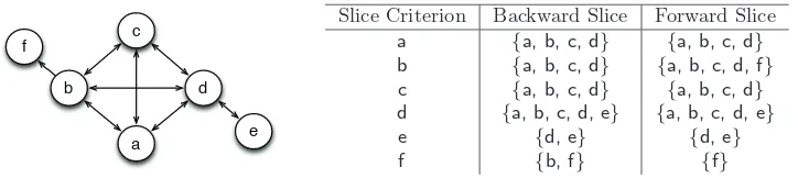
Figure 2: Backward slice inclusion relationship for Figure 1
and the edges represent the backward slice inclusion relationship from Figure 1. The table on the right of Figure 2 also gives the forward slice inclusions for
the statements. All other statements inP, which do not define a variable, are
ignored. In the diagram,xdepends ony(y∈BSlice(x)) is represented byy→x.
The diagram shows two instances of dependence intransitivity inP. Althoughb
depends on nodesa, c, and d, node f, which depends onb, does not depend on
a, c,ord. Similarly,ddepends onebuta, b,and c, which depend onddo not
depend one.
2.2. Slice-based Clusters
A slice-based cluster is a maximal set of vertices included in each others
slice. The following definition essentially instantiates Definition 1 usingBSlice.
Because x∈BSlice(y) ⇔y ∈ FSlice(x) the dual of this definition using FSlice
is equivalent. Where such a duality does not hold, both definitions are given.
When it is important to differentiate between the two, the termsbackward and
forward will be added to the definition’s name as is done in this section.
Definition 2 (Backward-Slice MDS and Cluster [26])
Abackward-slice MDS is a set of SDG vertices,V, such that
∀x, y∈V :x∈BSlice(y).
A backward-slice cluster is a backward-slice MDS contained within no other backward-slice MDS.
In the example shown in Figure 2, the vertices representing the assignments to a, b, c and d are all in each others backward slices and hence satisfy the definition of a backward-slice cluster. These vertices also satisfy the definition of a forward-slice cluster as they are also in each others forward slices.
As dependence is not transitive, a statement can be in multiple slice-based
clusters. For example, in Figure 2 the statementsdandeare mutually
depen-dent upon each other and thus satisfy the definition of a slice-based cluster.
Statementdis also mutually dependent on statementsa, b, c, thus the set{a,
b, c, d}also satisfies the definition of a slice-based cluster. It can be shown that
the clustering problem reduces to the NP-Hardmaximum clique problem [23]
2.3. Same-Slice Clusters
An alternative definition uses thesame-slice relation in place of slice inclu-sion [10]. This relation replaces the need to check if two vertices are in each others slice with checking if two vertices have thesameslice. The result is cap-tured in the following definitions forsame-slice cluster. The first uses backward slices and the second forward slices.
Definition 3 (Same-Slice MDS and Cluster [26])
Asame-backward-slice MDS is a set of SDG vertices,V, such that
8x, y2V :BSlice(x) =BSlice(y).
Asame-backward-slice cluster is a same-backward-slice MDS contained within no other same-backward-slice MDS.
Asame-forward-slice MDS is a set of SDG vertices,V, such that
8x, y2V :FSlice(x) =FSlice(y).
Asame-forward-slice cluster is a same-forward-slice MDS contained within no other same-forward-slice MDS.
Because x 2BSlice(x) and x2 FSlice(x), two vertices that have the same slice will always be in each other’s slice. If slice inclusion were transitive, a backward-slice MDS (Definition 2) would be identical to a same-backward-slice MDS (Definition 3). However, as illustrated by the examples in Figure 1, slice inclusion is not transitive; thus, the relation is one of containment where every same-backward-slice MDS is also a backward-slice MDS but not necessarily a maximal one.
For example, in Figure 2 the set of vertices{a, b, c}form a same-backward-slice cluster because each vertex of the set yields the same backward same-backward-slice. Whereas the set of vertices {a, c} form a same-forward-slice cluster as they have the same forward slice. Although vertex d is mutually dependent with all vertices of either set, it doesn’t form the same-slice cluster with either set because it has additional dependence relationship with vertexe.
Although the introduction of same-slice clusters was motivated by the need for efficiency, the definition inadvertently introduced anexternalrequirement on the cluster. Comparing the definitions for slice-based clusters (Definition 2) and same-slice clusters (Definition 3), a slice-based cluster includes only theinternal requirement that the vertices of a cluster depend upon one another. However, a same-backward-slice cluster (inadvertently) adds to this internal requirement theexternalrequirement that all vertices in the cluster are a↵ected by the same vertices external to the cluster. Symmetrically, a same-forward-slice cluster adds theexternal requirement that all vertices in the cluster a↵ect the same vertices external to the cluster.
2.4. Coherent Dependence Clusters
are dependence clusters that include not only an internal dependence require-ment (each staterequire-ment of a cluster depends on all the other staterequire-ments of the cluster) but also an external dependence requirement. The external depen-dence requirement includes both that each statement of a cluster depends on the same statements external to the cluster and also that it influences the same set of statements external to the cluster. In other words, a coherent cluster is a set of statements that are mutually dependent and share identical extra-cluster dependence. Coherent clusters are defined in terms of the coherent MDS:
Definition 4 (Coherent MDS and Cluster [29]) Acoherent MDS is a set of SDG verticesV, such that
8x, y 2 V : x depends on a implies y depends on a and a depends on x impliesadepends ony.
Acoherent cluster is a coherent MDS contained within no other coherent MDS. The slice-based instantiation of coherent cluster employs both backwardand forward slices. The combination has the advantage that the entire cluster is both a↵ected by the same set of vertices (as in the case of same-backward-slice clusters) and also a↵ects the same set of vertices (as in the case of same-forward-slice clusters). The same-forward-slice-based instantiation yieldscoherent-slice clusters:
Definition 5 (Coherent-Slice MDS and Cluster [29]) Acoherent-slice MDS is a set of SDG vertices,V, such that
8x, y2V :BSlice(x) =BSlice(y)^FSlice(x) =FSlice(y)
A coherent-slice cluster is a coherent-slice MDS contained within no other coherent-slice MDS.
At first glance the use of both backward and forward slices might seem redundant becausex2BSlice(y),y 2 FSlice(x). This is true up to a point: for the internal requirement of a coherent-slice cluster, the use of eitherBSliceor FSlicewould suffice. However, the two are not redundant when it comes to the external requirements of a coherent-slice cluster. With a mutually-dependent cluster (Definition 1), it is possible for two vertices within the cluster to influence or be a↵ected by di↵erent vertices external to the cluster. Neither is allowed with a coherent-slice cluster. To ensure both external e↵ects are captured, both backward and forward slices are required.
2.5. Hashed based Coherent Slice Clusters
The computation of coherent-slice clusters (Definition 5) grows prohibitively expensive even for mid-sized programs where tens of gigabytes of memory are required to store the set of all possible backward and forward slices. The com-putation is cubic in time and quadratic in space. An approximation is employed to reduce the computation time and memory requirement. This approximation replaces comparison of slices with comparison of hash values, where hash values are used to summarize slice content. The result is the following approximation to coherent-slice clusters in whichHdenotes a hash function.
Definition 6 (Hash-Based Coherent-Slice MDS and Cluster [29]) Ahash-based coherent-slice MDS is a set of SDG vertices,V, such that
8x, y2V :H(BSlice(x)) =H(BSlice(y))^H(FSlice(x)) =H(FSlice(y)) Ahash-based coherent-slice clusteris a hash-based coherent-slice MDS contained within no other hash-based coherent-slice MDS.
The precision of this approximation is empirically evaluated in Section 3.3. From here on, the paper considers only hash-based coherent-slice clusters unless explicitly stated otherwise. Thus, for ease of reading, hash-based coherent-slice cluster is referred to simply ascoherent cluster.
2.6. Graph Based Cluster Visualization
This section describes two graph-based visualizations for dependence clus-ters. The first visualization, theMonotone Slice-size Graph(MSG) [10], plots a landscape of monotonically increasing slice sizes where the y-axis shows the size of each slice, as a percentage of the entire program, and the x-axis shows each slice, in monotonically increasing order of slice size. In an MSG, a de-pendence cluster appears as a sheer-drop cli↵face followed by a plateau. The visualization assists with the inherently subjective task of deciding whether a cluster is large (how long is the plateau at the top of the cli↵face relative to the surrounding landscape?) and whether it denotes a discontinuity in the depen-dence profile (how steep is the cli↵face relative to the surrounding landscape?). An MSG drawn using backward slice sizes is referred to as a backward-slice MSG (B-MSG), and an MSG drawn using forward slice sizes is referred to as a forward-slice MSG (F-MSG).
As an example, the open source calculator bccontains 9,438 lines of code represented by 7,538 SDG vertices. The B-MSG for bc, shown in Figure 3a, contains a large plateau that spans almost 70% of the MSG. Under the assump-tion that same slice size implies the same slice, this indicates a large same-slice cluster. However, “zooming” in reveals that the cluster is actually composed of several smaller clusters made from slices of very similar size. The tolerance implicit in the visual resolution used to plot the MSG obscures this detail.
(a) B-MSG (b) F-MSG
Figure 3: MSGs for the programbc.
ordered along thex-axis first according to their slice size, second according to their same-slice cluster size, and third according to the coherent cluster size. Three values are plotted on they-axis: slice sizes form the first landscape, and cluster sizes form the second and third. Thus, SCGs not only show the sizes of the slices and the clusters, they also show the relation between them and thus bring to light interesting links. Two variants of the SCG are considered: the backward-slice SCG (B-SCG) is built from the sizes of backward slices, same-backward-slice clusters, and coherent clusters, while the forward-slice SCG (F-SCG) is built from the sizes of forward slices, same-forward-slice clusters, and coherent clusters. Note that both backward and forward SCGs use the same coherent cluster sizes.
The B-SCG and F-SCG for the programbcare shown in Figure 4. In both graphs the slice size landscape is plotted using a solid black line, the same-slice cluster size landscape using a gray line, and the coherent cluster size landscape using a (red) broken line. The B-SCG (Figure 4a) shows thatbccontains two large same-backward-slice clusters consisting of almost 55% and almost 15% of the program. Surprisingly, the larger same-backward-slice cluster is composed of smaller slices than the smaller same-backward-slice cluster; thus, the smaller cluster has a bigger impact (slice size) than the larger cluster. In addition, the presence of three coherent clusters spanning approximately 15%, 20% and 30% of the program’s statements can also be seen.
2.7. Cluster Visualization Tool
(a) B-SCG (b) F-SCG Figure 4: SCGs for the programbc
n ~ 1a
n ~ 2a
n ~ 3a
n ~ 1b
n ~ 2b
n ~ 3b
n ~ 1c
n ~ 2c
n ~ 3c
Figure 5: Heat Map View forbc
abstraction, the cluster visualization tool decluvi [28] provides four views: a Heat Mapview and three di↵erent source-code views. The latter three include theSystem View, theFile View, and theSource View, which allow a program’s clusters to be viewed at increasing levels of detail. A common coloring scheme is used in all four views to help tie the di↵erent views together.
the left of the Heat Map, using one pixel per cluster, horizontal lines (limited to 100 pixels) show the number of clusters that exist for each cluster size. This helps identify cases where there are multiple clusters of the same size. For example, the single dot next to the labels1a,2aand3adepict that there is one cluster for each of the three largest sizes. A single occurrence is common for large clusters, but not for small clusters as illustrated by the long line at the top left of the Heat Map, which indicates multiple (uninteresting) clusters of size one.
To the right of the cluster counts is the actual Heat Map (color spectrum) showing cluster sizes from small to large reading from top to bottom using colors varying from blue to red. In gray scale this appear as shades of gray, with lighter shades (corresponding to blue) representing smaller clusters and darker shades (corresponding to red) representing larger clusters. Red is used for larger clusters as they are more likely to encompass complex functionality, making them more important “hot topics”.
A numeric scale on the right of the Heat Map shows the cluster size (mea-sured in SDG vertices). For programbc, the scale runs from 1–2432, depicting the sizes of the smallest cluster, displayed using light blue (light gray), and the largest cluster, displayed in bright red (dark gray).
Finally, on the right of the number scale, two slice size statistics are dis-played: |BSlice|and|FSlice|, which show the sizes of the backward and forward slices for the vertices that form a coherent cluster. The sizes are shown as a percentage of the SDG’s vertex count, with the separation of the vertical bars representing 10% increments. For example, Cluster 1’s BSlice(1b) and FSlice (1c) include approximately 80% and 90% of the program’s SDG vertices, re-spectively.
Turning todecluvi’s three source-code views, theSystem Viewis at the high-est level of abstraction. Each file containing executable source code is abstracted into a column. Forbcthis yields the nine columns seen in Figure 6. The name of the file appears at the top of each column, color coded to reflect the size of the largest cluster found within the file. The vertical length of a column represents the length of the corresponding source file. To keep the view compact, each line of pixels in a column summarizes multiple source lines. For moderate sized systems, such as the case studies considered herein, each pixel line represents about eight source code lines. The color of each line reflects the largest cluster found among the summarized source lines, with light gray denoting source code that does not include any executable code. Finally, the numbers at the bottom of each column indicate the presence of the top 10 clusters in the file, where 1 denotes the largest cluster and 10 is the 10th largest cluster. Although there may be other smaller clusters in a file, numbers are used to depict only the ten largest clusters because they are most likely to be of interest. In the case studies considered in Section 3, only the five largest coherent clusters are ever found to be interesting.
Figure 7: File View for the fileutil.c of Programbc. Each line of pixels corre-spond to one source code line. Blue (medium gray in black & white) represents lines with vertices belonging to the 2ndlargest cluster and red (dark gray) rep-resents lines with vertices belonging to the largest cluster. The rectangle marks functioninit gen, part of both clusters.
lines are indented to mimic the indentation of the source lines and the number of pixels used to draw each line corresponds to the number of characters in the represented source code line. This makes it easier to relate this view to actual source code. The color of a pixel line depicts the size of the largest coherent cluster formed by the SDG vertices from the corresponding source code line. Figure 7 shows the File View of bc’s file util.c, filtered to show only the two largest coherent clusters, while smaller clusters and non-executable lines are shown in light gray.
Figure 8: Source View showing function init gen in file util.c of Program bc. Thedecluvioptions are set to filter out all but the two largest clusters thus blue (medium gray in black & white) represents lines from the 2ndlargest cluster and red (dark gray) lines from the largest cluster. All other lines including those with no executable code are shown in light gray.
concrete view that maps the clusters onto actual source code lines. The lines are displayed in the same spatial context in which they were written, line color depicts the size of the largest cluster to which the SDG vertices representing the line belong. Figure 8 shows Lines 241–257 ofbc’s fileutil.c, which has again been filtered to show only the two largest coherent clusters. The lines of code whose corresponding SDG vertices are part of the largest cluster are shown in red (dark gray) and those lines whose SDG vertices are part of the second largest cluster are shown in blue (medium gray). Other lines that do not include any executable code or whose SDG vertices are not part of the two largest clusters are shown in light gray. On the left of each line is aline tag with the format a:b|c/d, which represents the line number (a), the cluster number (b), and an identificationc/dfor the cth ofdclusters having a given size. For example, in Figure 8, Lines 250 and 253 are both part of a 20th largest cluster (clusters with same size have the same rank) as indicated by the value ofb; however they belong to di↵erent clusters as indicated by the di↵ering values ofcin their line tags.
indistinguishable.
3. Empirical Evaluation
This section presents the empirical evaluation into the existence and impact of coherent dependence clusters. The section first discusses the experimental setup and the subject programs included in the study. It then presents two validation studies, the first on the use of CodeSurfer’s pointer analysis, and, the second on the use of hashing to summarize slices for efficient cluster iden-tification. The section then quantitatively considers the existence of coherent dependence clusters and identifies patterns of clustering within the programs. This is followed by a series of four case studies, where qualitative analysis, aided bydecluvi, is used to highlight how knowledge of clusters can aid a software en-gineer. Finally, inter-cluster dependence and threats to validity are considered. More formally, the empirical evaluation addresses the following research ques-tions:
RQ1 Does increased pointer analysis precision result in smaller coherent clus-ters?
RQ2 Does hashing provide a sufficient summary of a slice to allow comparing hash values to replace comparing slices?
RQ3 Do large coherent clusters exist in production source code? RQ4 Which patterns of clustering can be identified?
RQ5 Can analysis of coherent clusters reveal structures within a program? RQ6 Does dependence between coherent clusters induce larger dependence
structures?
The first two research questions (RQ1andRQ2) provide empirical verifica-tion for the results subsequently presented. RQ1establishes the impact of the data flow analysis quality used by the slicing tool. WhereasRQ2is the foun-dation for the remaining empirical study because it establishes that the hash function for approximating slice content is sufficiently precise. If the static slices produced by the slicer are overly conservative or if the slice approximation is not sufficiently precise, then the results presented will not be reliable. Fortunately, the results provide confidence that the slice precision and hashing accuracy are sufficient.
SDG Largest
Program C LoC SLoC ELoC vertex Total Coherent Description Files count Slices Cluster Size
a2ps 79 46,620 22,117 18,799 224,413 97,170 8% ASCII to Postscript
acct 7 2,600 1,558 642 7,618 2,834 11% Process monitoring
acm 114 32,231 21,715 15,022 159,830 63,014 43% Flight simulator anubis 35 18,049 11,994 6,947 112,282 34,618 13% SMTP messenger
archimedes 1 787 575 454 20,136 2,176 4% Semiconductor device simulator barcode 13 3,968 2,685 2,177 16,721 9,602 58% Barcode generator
bc 9 9,438 5,450 4,535 36,981 15,076 32% Calculator
byacc 12 6,373 5,312 4,688 45,338 16,590 7% Parser generator cflow 25 12,542 7,121 5,762 68,782 24,638 8% Control flow analyzer combine 14 8,202 6,624 5,279 49,288 29,118 15% File combinator
copia 1 1,168 1,111 1,070 42,435 6,654 48% ESA signal processing code
cppi 13 6,261 1,950 2,554 17,771 10,280 13% C preprocessor formatter
ctags 33 14,663 11,345 7,383 152,825 31,860 48% Ctagging
diction 5 2,218 1,613 427 5,919 2,444 16% Grammar checker
di↵utils 23 8,801 6,035 3,638 30,023 16,122 44% File di↵erencing
ed 8 2,860 2,261 1,788 35,475 11,376 55% Line text editor
enscript 22 14,182 10,681 9,135 67,405 33,780 19% File converter findutils 59 24,102 13,940 9,431 102,910 41,462 22% Line text editor
flex 21 23,173 12,792 13,537 89,806 37,748 16% Lexical Analyzer
garpd 1 669 509 300 5,452 1,496 14% Address resolved
gcal 30 62,345 46,827 37,497 860,476 286,000 62% Calendar program
gnuedma 1 643 463 306 5,223 1,488 44% Development environment
gnushogi 16 16,301 11,664 7,175 64,482 31,298 40% Japanese chess indent 8 6,978 5,090 4,285 24,109 7,543 52% Text formatter
less 33 22,661 15,207 9,759 451,870 33,558 35% Text reader
spell 1 741 539 391 6,232 1,740 20% Spell checker
time 6 2,030 1,229 433 4,946 3,352 4% CPU resource measure
userv 2 1,378 1,112 1,022 15,418 5,362 9% Access control
wdi↵ 4 1,652 1,108 694 10,077 2,722 6% Di↵front end
which 6 3,003 1,996 753 8,830 3,804 35% Unix utility
Average 20 11,888 7,754 5,863 91,436 28,831 27% Table 1: Subject programs
These results motivate the remaining research questions. Having demon-strated that our technique is suitable for finding coherent clusters and that such clusters are sufficiently widespread to be worthy of study, we investigate spe-cific coherent clusters in detail. RQ4asks whether there are common patterns of clustering in the programs studied andRQ5asks whether these clusters reveal aspects of the underlying logical structure of programs. Finally,RQ6looks ex-plicitly at inter-cluster dependency relationships and considers areas of software engineering where they may be of interest.
3.1. Experimental Subjects and Setup
than the other source code measures because they reflect SLoC for the particular preprocessed version of the program considered by CodeSurfer.
The data and visualizations presented in this paper are generated from slices taken with respect to source-code representing SDG vertices. This excludes pseudo vertices introduced into the SDG, to represent, for example, global vari-ables, which are modeled as additional pseudo parameters by CodeSurfer. Thus in Table 1 total slices is smaller than the SDG vertex count. Cluster sizes are also measured in terms of source-code representing SDG vertices, which is more consistent than using lines of code as it is not influenced by blank lines, com-ments, statements spanning multiple lines, multiple statements on one line, or compound statements.
The slices along with the mapping between the SDG vertices and the actual source code is extracted from the mature and widely used slicing tool CodeSurfer (version 2.1). The cluster visualizations were generated bydecluviusing data ex-tracted from CodeSurfer. Thedecluvisystem along with scheme scripts for data acquisition and pre-compiled datasets for several open-source programs can be downloaded fromhttp://www.cs.ucl.ac.uk/staff/s.islam/decluvi.html 3.2. CodeSurfer Pointer Analysis
Recall that the definition of a coherent dependence cluster is based on an underlying depends-on relation, which is approximated using program slicing. Pointer analysis plays a key role in the precision of slicing. This section presents a study on the e↵ect of various levels of pointer-analysis precision on the size of the coherent clusters. It addresses research question RQ1 by considering whether more sophisticated pointer analysis results in more precise slices and hence smaller clusters. There is no automatic way to determine whether the slices are correct and precise, we use slice size as a measure of conciseness and thus precision.
Program Average Slice Size Max Slice Size Average Cluster Size MaxCluster Size
L M H L M H L M H L M H
a2ps 25223 23085 20897 45231 44139 43987 2249 1705 711 10728 9295 4002
acct 763 700 621 1357 1357 1357 79 66 40 272 236 162
acm 19083 17997 16509 29403 28620 28359 3566 3408 4197 9356 9179 10809
anubis 11120 10806 9085 16548 16347 16034 939 917 650 2708 2612 2278
archimedes 113 113 113 962 962 962 3 3 3 39 39 39
barcode 3523 3052 2820 4621 4621 4621 1316 1870 1605 2463 2970 2793
bc 5278 5245 5238 7059 7059 7059 1185 1188 1223 2381 2384 2432
byacc 3087 2936 2886 9036 9036 9036 110 110 103 583 583 567
cflow 7314 5998 5674 11856 11650 11626 865 565 246 3060 2191 1097
combine 3512 3347 3316 13448 13448 13448 578 572 533 2252 2252 2161
copia 1844 1591 1591 3273 3273 3273 1566 1331 1331 1861 1607 1607
cppi 1509 1352 1337 4158 4158 4158 196 139 139 825 663 663
ctags 12681 11663 11158 15483 15475 15475 7917 4199 3955 11080 7905 7642
diction 421 392 387 1194 1194 1194 46 37 37 217 196 196
di↵utils 5049 4546 4472 7777 7777 7777 3048 1795 1755 4963 3596 3518
ed 4203 3909 3908 5591 5591 5591 2099 1952 1952 3281 3146 3146
enscript 7023 6729 6654 16130 16130 16130 543 554 539 3140 3242 3243 findutils 7020 6767 5239 11075 11050 11050 1969 1927 1306 4489 4429 2936
flex 9038 8737 8630 17257 17257 17257 622 657 647 3064 3064 3064
garpd 284 242 224 628 628 628 32 31 29 103 103 103
gcal 132860 123438 123427 142739 142289 142289 40885 40614 40614 93541 88532 88532
gnuedma 385 369 368 730 730 368 178 176 174 333 331 330
gnushogi 9569 9248 9141 14726 14726 14726 1577 2857 2820 3787 6225 6179
indent 4104 4058 4045 5704 5704 5704 2036 2032 1985 3402 3399 3365
less 13592 13416 13392 16063 16063 16063 4573 3074 3035 7945 5809 5796
spell 359 293 291 845 845 845 58 31 48 199 128 174
time 201 161 158 730 730 730 4 3 3 35 33 33
userv 1324 972 964 2721 2662 2662 69 32 53 268 154 240
wdi↵ 687 582 561 2687 2687 2687 33 21 19 184 158 158
which 1080 1076 1070 1744 1744 1744 413 413 410 798 798 793
Table 2: CodeSurfer pointer analysis settings
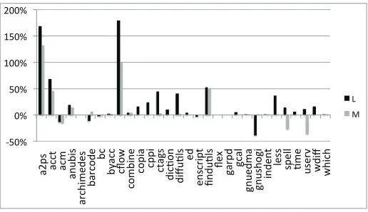
largest cluster size deviation are visualized in Figures 9 and 10. The graphs use the High setting as the base line and show the percentage deviation when using the Low and Medium settings.
Figure 9 shows the average slice size deviation when using the lower two set-tings compared to the highest. On average, the Low setting produces slices that are 14% larger than the High setting. Programuservhas the largest deviation of 37% when using the Low setting. For example, inuservthe minimal pointer analysis fails to recognize that the function pointeroipcan never point to func-tionssighandler alrmandsighandler childand includes them as called functions at call sites using*oip, increasing slice size significantly. In all 30 programs, the Low setting yields larger slices compared to the High setting.
' $' ' $' !' !$' "' "$' #'
!
Figure 9: Percentage deviation of average slice size for Low and Medium CodeSurfer pointer analysis settings
# & & # & ! & !# & " &
"
[image:20.612.178.435.122.274.2]
Figure 10: Percentage deviation of largest cluster size for Low and Medium CodeSurfer pointer analysis settings
fields (options, regex map, stat buf andstate) offindutilsare lumped together as if
each structure were a scalar variable, resulting in larger, less precise, slices. Figure 10 visualizes the deviation of the largest coherent cluster size when using the lower two settings compared to the highest. The graph shows that the size of the largest coherent clusters found when using the lower settings is larger in most of the programs. On average there is a 22% increase in the size of the largest coherent cluster when using the Low setting and a 10% increase
when using the Medium setting. Ina2psandcflowthe size of the largest cluster
increases over 100% when using the Medium setting and over 150% when using the Low setting. The increase in slice size is expected to result in larger clusters due to the loss of precision.
[image:20.612.177.435.320.469.2]Low Medium High (a)a2ps
Low Medium High
(b)cflow
Low Medium High
(c)acm
graphs it is seen that the slice sizes get smaller and have increased steps in the (black) landscape indicating that they become more precise. The red landscape shows that there is a large coherent cluster detected when using the Low setting running from approx. 60% to 85% on thex-axis. This cluster drops in size when using the Medium setting. At the High setting this coherent clusters breaks up into multiple smaller clusters. In this case, a drop in the cluster size also leads to breaking of the cluster in to multiple smaller clusters.
In the SCGs forcflow(Figure 11b) a similar drop in the slice size and cluster size is observed. However, unlikea2psthe large coherent cluster does not split into smaller clusters but only drops in size. The largest cluster when using the Low setting runs from 60% to 85% on the x-axis. This cluster reduces in size and shifts position running 30% to 45%x-axis when using the Medium setting. The cluster further drops in size down to 5% running 25% to 30% on thex-axis when using the High setting. In this case the largest cluster has a significant drop in size but doesn’t split into multiple smaller clusters.
f6(x){
f = *p(42, 4); return f; }
Figure 12: replacement coherent cluster example
Surprisingly, Figure 10 also shows seven programs where the largest coherent cluster size actually increases when using the highest pointer analysis setting on CodeSurfer. Figure 11c shows the B-SCGs foracmwhich falls in this category. This counter-intuitive result is seen only when the more precise analysis deter-mines that certain functions cannot be called and thus excludes them from the slice. Although in all such instances slices get smaller, the clusters may grow if the smaller slices match other slices already forming a cluster.
For example, consider replacing functionf6in Figure 1 with the code shown in Figure 12, wherefdepends on a function call to a function referenced through the function pointerp. Assume that the highest precision pointer analysis deter-mines thatpdoes not point tof2and therefore there is no call tof2or any other function fromf6. The higher precision analysis would therefore determine that the forward slices and backward slices of a, b andcare equal, hence grouping these three vertices in a coherent cluster. Whereas the lower precision is unable to determine thatp cannot point tof2, the backward slice on f will conserva-tively includeb. This will lead the higher precision analysis to determine that the set of vertices{a, b, c} are one coherent cluster whereas the lower precision analysis include only set of vertices{a, c}in the same coherent cluster.
Be-cause it gives the most precise slices and most accurate clusters, the remainder of the paper uses the highest CodeSurfer pointer analysis setting.
3.3. Validity of the Hash Function
This section addresses research question RQ2: Does hashing provide a suf-ficient summary of a slice to allow comparing hash values to replace comparing slices? The section validates the use of comparing slice hash values in lieu of comparing actual slice content. The use of hash values to represent slices re-duce both the memory requirement and run-time, as it is no longer necessary to store or compare entire slices. The hash function, denotedHin Definition 6, determines a hash value for a slice based on the unique vertex ids assigned by CodeSurfer. Validation of this approach is needed to confirm that the hash values provide a sufficiently accurate summary of slices to support the correct partitioning of SDG vertices into coherent clusters. Ideally, the hash function would produce a unique hash value for each distinct slice. The validation study aims to find the number of unique slices for which the hash function successfully produces an unique hash value.
For the validation study we chose 16 programs from the set of 30 subject programs. The largest programs were not included in the validation study to make the study-time manageable. Results are based on both the backward and forward slices for every vertex of these 16 programs. To present the notion of precision we introduce the following formalization. Let V be the set of all source-code representing SDG vertices for a given program P and U S denote the number ofunique slices: U S=|{BSlice(x) :x2V}|+|{FSlice(x) :x2V}|. Note that if all vertices have the same backward slice then{BSlice(x) :x2V} is a singleton set. Finally, letU H be the number ofunique hash-values,U H = |{H(BSlice(x)) :x2V}|+|{H(FSlice(x)) :x2V}|.
The accuracy of hash functionHis given as Hashed Slice Precision,HSP = U H/U S. A precision of 1.00 (U S = U H) means the hash function is 100% accurate (i.e., it produces a unique hash value for every distinct slice) whereas a precision of 1/U S means that the hash function produces the same hash value for every slice leavingU H = 1.
Table 3 summarizes the results. The first column shows each program. The second and the third columns report the values ofU SandU H respectively. The fourth column reportsHSP, the precision attained using hash values to compare slices. Considering all 78,587 unique slices the hash function produced unique hash values for 74,575 of them, resulting in an average precision of 94.97%. In other words, the hash function fails to produce unique hash values for just over 5% of the slices. Considering the precision of individual programs, five of the programs have a precision greater than 97%, while the lowest precision, for findutils, is 92.37%. This is, however, a significant improvement over previous use of slice size as the hash value, which is only 78.3% accurate [10].
Unique Hashed Hash Hash Unique Hash Slice Cluster Cluster Precision
Slices values Precision Count Count Clusters Program (U S) (U H) (HSP) (CC) (HCC) (HCP)
acct 1,558 1,521 97.63% 811 811 100.00%
barcode 2,966 2,792 94.13% 1,504 1,504 100.00%
bc 3,787 3,671 96.94% 1,955 1,942 99.34%
byacc 10,659 10,111 94.86% 5,377 5,377 100.00% cflow 16,584 15,749 94.97% 8,457 8,452 99.94%
copia 3,496 3,398 97.20% 1,785 1,784 99.94%
ctags 8,739 8,573 98.10% 4,471 4,470 99.98%
di↵utils 5,811 5,415 93.19% 2,980 2,978 99.93%
ed 2,719 2,581 94.92% 1,392 1,390 99.86%
findutils 9,455 8,734 92.37% 4,816 4,802 99.71%
garpd 808 769 95.17% 413 411 99.52%
indent 3,639 3,491 95.93% 1,871 1,868 99.84%
time 1,453 1,363 93.81% 760 758 99.74%
userv 3,510 3,275 93.30% 1,827 1,786 97.76%
wdi↵ 2,190 2,148 98.08% 1,131 1,131 100.00%
which 1,213 1,184 97.61% 619 619 100.00%
Sum 78,587 74,575 – 40,169 40,083 –
Average 4,912 4,661 94.97% 2,511 2,505 99.72%
Table 3: Hash function validation
hash values matching those from another vertex with di↵erent slices is less than that of a single collision. Extending U S and U H to clusters, Columns 5 and 6 (Table 3) report CC, the number of coherent clusters in a program and HCC, the number of coherent clusters found using hashing. The final column shows the precision attained using hashing to identify clusters,HCP = HCC/CC. The results show that of the 40,169 coherent clusters, 40,083 are uniquely identified using hashing, which yields a precision of 99.72%. Five of the programs show total agreement, furthermore for each programHCP is over 99%, except foruserv, which has the lowest precision of 97.76%. This can be attributed to the large percentage (96%) of single vertex clusters inuserv. The hash values for slices taken with respect to these single-vertex clusters have a higher potential for collision leading to a reduction in overall precision. In summary, this study provides an affirmative answer to RQ2. The hash-based approximation is sufficiently accurate. Comparing hash values can replace the need to compare actual slices.
3.4. Do large coherent clusters occur in practice?
! " # $ %
[image:25.612.143.472.131.281.2]
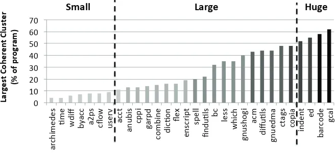
Figure 13: Size of largest coherent cluster
To assess if a program includes a largecoherent cluster, requires making a
judgement concerning what threshold constitutes large. Following prior empiri-cal work [10, 26, 28, 29], a threshold of 10% is used. In other words, a program is said to contain a large coherent cluster if 10% of the program’s SDG vertices produce the same backward slice as well as the same forward slice.
Figure 13 shows the size of the largest coherent cluster found in each of the 30 subject programs. The programs are divided into 3 groups based on the size of the largest cluster present in the program.
Small: Smallconsists of seven programs none of which have a coherent clus-ter constituting over 10% of the program vertices. These programs are
archimedes, time, wdiff, byacc, a2ps, cflowand userv. Although it may be in-teresting to study why large clusters are not present in these programs, this paper focuses on studying the existence and implications of large co-herent clusters.
Large: This group consists of programs that have at least one cluster with size 10% or larger. As there are programs containing much larger coherent clusters, a program is placed in this group if it has a large cluster between the size 10% and 50%. Over two-thirds of the programs studied fall in this category.
The program at the bottom of this group (acct) has a coherent cluster
of size 11% and the largest program in this group (copia) has a coherent
cluster of size 48%. We present both these programs as case studies and discuss their clustering in detail in Sections 3.6.1 and 3.6.4, respectively.
The programbcwhich has multiple large clusters with the largest of size
32% falls in the middle of this group and is also presented as a case study in Section 3.6.3.
whose size is over 50%. Out of the 30 programs 4 fall in this group. These programs are indent, ed, barcode and gcal. From this group, we present indentas a case study in Section 3.6.2.
In summary all but 7 of the 30 subject programs contain a large coherent cluster. Therefore, over 75% of the subject programs contain a coherent cluster of size 10% or more. Furthermore, half the programs contain a coherent cluster of at least 20% in size. It is also interesting to note that although this grouping is based only on the largest cluster, many of the programs contain multiple large coherent clusters. For example,ed, ctags, nano, less, bc, findutils, flexandgarpdall have multiple large coherent clusters. It is also interesting to note that there is no correlation between a program’s size (measured in SLoC) and the size of its largest coherent cluster. For example, in Table 1 two programs of very di↵erent sizes,cflowand userv, have similar largest-cluster sizes of 8% and 9%, respectively. Whereas programsacct anded, of similar size, have very di↵erent largest coherent clusters of sizes 11% and 55%.
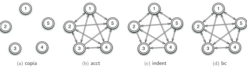
archimedes time wdi↵ byacc
a2ps cflow userv
Figure 14: Programs withsmall coherent clusters
Therefore as an affirmative answer to RQ3, the study finds that 23 of the 30 programs studied have a large coherent cluster. Some programs also have a huge cluster covering over 50% of the program vertices. Furthermore, the choice of 10% as a threshold for classifying a cluster as large is a relatively conservative choice. Thus, the results presented in this section can be thought of as a lower bound to the existence question.
3.5. Patterns of clustering
acct anubis cppi garpd
combine diction flex enscript
spell findutils bc less
which gnushogi acm diffutils
[image:27.612.97.523.133.519.2]gnuedma ctags copia
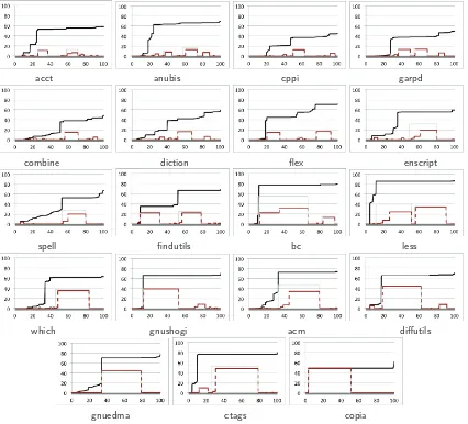
Figure 15: Programs withlargecoherent clusters
indent ed barcode gcal
[image:27.612.101.520.561.642.2]Figure 14 shows SCGs for the seven programs of the small group. In the SCGs of the first three programs (archimedes, timeandwdi↵) only a small coherent cluster is visible in the red landscape. In the remaining four programs, the red landscape shows the presence of multiple small coherent clusters. It is very likely that, similar to the results of the case studies presented later, these clusters also depict logical constructs within each program.
Figure 15 shows SCGs of the 19 programs that have at least one large, but not huge, coherent cluster. That is, each program has at least one coherent cluster covering 10% to 50% of the program. Most of the programs have multiple coherent clusters as is visible on the red landscape. Some of these have only one large cluster satisfying the definition oflarge, such asacct. The clustering ofacct is discussed in further detail in Section 3.6.1. Most of the remaining programs are seen to have multiple large clusters such asbc, which is also discussed in further detail in Section 3.6.3. The presence of multiple large coherent cluster hints that the program consists of multiple functional components. In three of the programs (which, gnuedmaandcopia) the landscape is completely dominated by a single large coherent cluster. In which and gnuedma this cluster covers around 40% of the program vertices whereas incopiathe cluster covers 50%. The presence of a single large dominating cluster points to a centralized functionality or structure being present in the program. Copiais presented as a case study in Section 3.6.4 where its clustering is discussed in further detail.
Finally, SCGs for the four programs that contain huge coherent clusters (covering over 50%) are found in Figure 16. In all four landscapes there is a very large dominating cluster with other smaller clusters also being visible. This pattern supports the conjecture that the program has one central structure or functionality which consists of most of the program elements, but also has additional logical constructs that work in support of the central idea. Indent is one program that falls in this category and is discussed in further detail in Section 3.6.2.
As an answer toRQ4, the study finds that most programs contain multiple coherent clusters. Furthermore, the visual study reveals that a third of the programs have multiple large coherent clusters. Only three programs copia, gnuedma, andwhichshow the presence of only a single (overwhelming) cluster.
Having shown that coherent clusters are prevalent in programs and that most programs have multiple significant clusters, it is our conjecture that these clusters represent high-level functional components of programs and hence rep-resent the systems logical structure. The following sections prep-resent a series of four case studies where such mappings are discussed in details.
3.6. Coherent Cluster and program decomposition
group. Each of the three programs from thelarge group were chosen because it exhibits specific patterns. Acct has multiple coherent clusters visible in its profile and has the smallest large cluster in the group, bc has multiple large coherent clusters, andcopia has only a single large coherent cluster dominating the entire landscape.
3.6.1. Case Study: acct
The first of the series of case studies is acct, an open-source program used for monitoring and printing statistics about users and processes. The program acctis one of the smaller programs with 2,600 LoC and 1,558 SLoC from which CodeSurfer produced 2,834 slices. The program has sevenCfiles, two of which, getopt.candgetopt1.c, contain only conditionally included functions. These func-tions provide support for command-line argument processing and are included if needed library code is missing.
Table 4 shows the statistics for the five largest clusters of acct. Column 1 gives the cluster number, where1is the largest and5is the 5thlargest cluster measured using the number of vertices. Columns 2 and 3 show the size of the cluster as a percentage of the program’s vertices and actual vertex count, as well as the line count. Columns 4 and 5 show the number of files and functions where the cluster is found. The cluster sizes range from 11.4% to 2.4%. These five clusters can be readily identified in the Heat-Map visualization (not shown) ofdecluvi. The rest of the clusters are very small (less than 2% or 30 vertices) in size and are thus of little interest.
Cluster Cluster Size Files Functions % vertices/lines spanned spanned
1 11.4% 162/88 4 6
2 7.2% 102/56 1 2
3 4.9% 69/30 3 4
4 2.8% 40/23 2 3
5 2.4% 34/25 1 1
Table 4: acct’s top five clusters
The B-SCG foracct(row one of Figure 15) shows the existence of these five coherent clusters along with other same-slice clusters. Splittingof the same-slice cluster is evident in the SCG. Splitting occurs when the vertices of a same-slice cluster become part of di↵erent coherent clusters. This happens when vertices have either the same backward slice or the same forward slice but not both. In acct’s B-SCG the vertices of the largest same-backward-slice cluster spanning thex-axis from 60% to 75% are not part of the same coherent cluster. This is because the vertices do not share the same forward slice. This splitting e↵ect is common among the programs studied.
ac.c, and hashtab.c), the 4th largest cluster spans two files (ac.cand hashtab.c), while the 5thlargest cluster includes parts ofac.conly.
The largest cluster ofacctis spread over six functions,log in,log out,file open, file reader get entry, bad utmp record and utmp get entry. These functions are re-sponsible forputting accounting records into the hash tableused by the program, accessing user-defined files, andreading entriesfrom the file. Thus, the purpose of the code in this cluster is to track user login and logout events.
The second largest cluster is spread over two functions hashtab create and hashtab resize. These functions are responsible forcreating fresh hash tables and resizing existing hash tableswhen the number of entries becomes too large. The purpose of the code in this cluster is the memory management in support of the program’s main data structure.
The third largest cluster is spread over four functions: hashtab set value, log everyone out,update user time, andhashtab create. These functions are respon-sible for setting values of an entry, updating all the statistics for users, and resetting the tables. The purpose of the code from this cluster is the modifica-tion of the user accounting data.
The fourth cluster is spread over three functions: hashtab delete,do statistics, andhashtab find. These functions are responsible forremoving entries from the hash table,printing out statisticsfor users andfinding entriesin the hash table. The purpose of the code from this cluster is maintaining user accounting data and printing results.
The fifth cluster is contained within the functionmain. This cluster is formed due to the use of a while loop containing various cases based on input to the program. Because of the conservative nature of static analysis, all the code within the loop is part of the same cluster.
Finally, it is interesting to note that functions from the same file or with similar names do not necessarily belong to the same cluster. Although six of the functions considered above have the common prefix “hashtab”, these functions are not part of the same cluster. Instead the functions that work together to provide a particular functionality are found in the same cluster. This case study provides an affirmative answer to RQ5. For acct, each of the top five clusters maps to specific functionality, which interestingly is not revealed simply from studying the names of the artifacts.
3.6.2. Case Study: indent
The next case study usesindent to further support to the answer found for RQ5in theacctcase study. The characteristics ofindentare very di↵erent from those ofacctasindenthas a very large dominant coherent cluster (52%) whereas accthas multiple smaller clusters with the largest being 11%. We includeindent as a case study to ensure that the answer for RQ5 is derived from programs with di↵erent cluster profiles and sizes giving confidence as to the generality of the answer.
Cluster Cluster Size Files Functions % vertices/lines spanned spanned
1 52.1% 3930/2546 7 54
2 3.0% 223/136 3 7
3 1.9% 144/72 1 6
4 1.3% 101/54 1 5
5 1.1% 83/58 1 1
Table 5: indent’s top five clusters
Indenthas one extremely large coherent cluster that spans 52.1% of the pro-gram’s vertices. The cluster is formed of vertices from 54 functions spread over 7 source files. This cluster captures most of the logical functionalities of the program. Out of the 54 functions, 26 begin with the common prefix of “handle token”. These 26 functions are individually responsible for handling a specific token during the formatting process. For example, handle token colon, handle token comma, handle token comment, andhandle token lbraceare responsible for handling the colon, comma, comment, and left brace tokens, respectively.
This cluster also includes multiple handler functions that check the size of the code and labels being handled, such ascheck code sizeandcheck lab size. Oth-ers, such assearch brace, sw bu↵er, print comment, andreduce, help with tracking braces and comments in code. The cluster also spans the main loop ofindent (indent main loop) that repeatedly calls the parser functionparse.
Finally, the cluster consists of code for outputting formatted lines such as the functionsbetter break, computer code target, dump line, dump line code, dump line label, inhibit indenting, is comment start, output line length and slip horiz space, and ones that perform flag and memory management (clear buf break list, fill bu↵er and set priority).
Cluster 1 therefore consists of the main functionality of this program and provides support forparsing, handling tokens, associated memory management, and output. The parsing, handling of individual tokens and associated mem-ory management are highly inter-twined. For example, the handling of each individual token is dictated by operations ofindentand closely depends on the parsing. This code cannot easily be decoupled and, for example, reused. Sim-ilarly the memory management code is specific to the data structures used by indent resulting in these many logical constructs to become part of the same cluster.
The second largest coherent cluster consists of 7 functions from 3 source files. These functions handle the arguments and parameters passed to indent. For example, set option and option prefix along with the helper function eqin to check and verify that the options or parameters passed toindentare valid. When options are specified without the required arguments, the function arg missing produces an error message by invoking usage followed by a call to DieError to terminate the program.
warrant a detailed discussion. Cluster 3 includes 6 functions that generate numbered/un-numbered backup for subject files. Cluster 4 has functions for reading and ignoring comments. Cluster 5 consists of a single function that reinitializes the parser and associated data structures.
The case study ofindentfurther illustrates that coherent clusters can capture the program’s logical model and finds an affirmative answer to research question RQ5. However, in cases such as this where the internal functionality is tightly knit, a single large coherent clusters maps to the program’s core functionality.
3.6.3. Case Study: bc
The third case study in this series is bc, an open-source calculator, which consists of 9,438 LoC and 5,450 SLoC. The program has nineCfiles from which CodeSurfer produced 15,076 slices (backward and forward).
Analyzingbc’s SCG (row 3, Figure 15), two interesting observations can be made. First, bc contains two large same-backward-slice clusters visible in the light gray landscapes as opposed to the three large coherent clusters. Second, looking at the B-SCG, it can be seen that the x-axis range spanned by the largest same-backward-slice cluster is occupied by the top two coherent clusters shown in the dashed red (dark gray) landscape. This indicates that the same-backward-slice cluster splits into the two coherent clusters.
The statistics forbc’s top five clusters are given in Table 6. Sizes of these five clusters range from 32.3% through to 1.4% of the program. Clusters six onwards are less than 1% of the program. Decluvi’s Heat Map View forbc (Figure 5) clearly shows the presence of these five clusters. The Project View (Figure 6) shows their distribution over the source files.
Cluster Cluster Size Files Functions % vertices/lines spanned spanned
1 32.3% 2432/1411 7 54
2 22.0% 1655/999 5 23
3 13.3% 1003/447 1 15
4 1.6% 117/49 1 2
5 1.4% 102/44 1 1
Table 6: bc’s top five clusters
fromutil.care employed. Only five lines of code inexecute.care also part of Clus-ter 2 and are used forflushing output andclearing interrupt signals. The third cluster is completely contained within the filenumber.c. It encompasses func-tions such as bc do sub, bc init num, bc do compare, bc do add, bc simp mul, bc shift addsub, and bc rm leading zeros, which are responsible forinitializing bc’s number formatter, performing comparisons, modulo and other arithmetic operations. Clusters 4 and 5 are also completely contained within number.c. These clusters encompass functions to performbcd operations for base ten num-bers andarithmetic division, respectively.
The results of the cluster visualizations forbcreveal its high-level structure. This aids an engineer in understanding how the artifacts (e.g., functions and files) of the program interact. The visualization of the clustering thus aids in program comprehension and provides further support forRQ5.
The following discussion illustrates a side-e↵ect of decluvi’s multi-level vi-sualization, how it can help find potential problems with the structure of a program. Util.c consists of small utility functions called from various parts of the program. This file contains code from Clusters 1 and 2 (Figure 6). Five of the utility functions belong with Cluster 1, while six belong with Cluster 2. Furthermore, Figure 7 shows that the distribution of the two clusters in red (dark gray) and blue (medium gray) within the file are well separated.
Both clusters do not occur together inside any function with the exception ofinit gen(highlighted by the rectangle in first column of Figure 7). The other functions ofutil.cthus belong to either Cluster 1 or Cluster 2. Separating these utility functions into two separate source files where each file is dedicated to functions belonging to a single cluster would improve the code’s logical separa-tion and file-level cohesion. This would make the code easier to understand and maintain at the expense of a very simple refactoring. In general, this example illustrates howDecluvivisualization can provide an indicator of potential points of code degradation during evolution.
Finally, the Code View for functioninit genshown in Figure 8 includes Lines 244, 251, 254, and 255 in red (dark gray) from Cluster 1 and Lines 247, 248, 249, and 256 in blue (medium gray) from Cluster 2. Other lines, shown in light gray, belong to smaller clusters and lines containing no executable code. Ide-ally, clusters should capture a particular functionality; thus, functions should generally not contain code from multiple clusters (unless perhaps the clusters are completely contained within the function). Functions with code from multi-ple clusters reduce code separation (hindering comprehension) and increase the likelihood of ripple-e↵ects [16]. Like other initialization functions, bc’s init gen form an exception to this guideline.
This case study not only provides an affirmative answer to research question RQ5, but also illustrates that the visualization is able to reveal structural defects in programs.
3.6.4. Case Study: copia
Cluster Cluster Size Files Functions number % vertices/lines spanned spanned
1 48% 1609/882 1 239
2 0.1% 4/2 1 1
3 0.1% 4/2 1 1
4 0.1% 4/2 1 1
5 0.1% 2/1 1 1
Table 7: copia’s top five clusters
(a)Original (b)Modified
Figure 17: SCGs for the programcopia
this series of case studies with 1,168 LoC and 1,111 SLoC all in a singleCfile. Its largest coherent cluster covers 48% of the program. The program is at the top of the group with large coherent clusters. CodeSurfer extracts 6,654 slices (backward and forward).
The B-SCG for copia is shown in Figure 17a. The single large coherent cluster spanning 48% of the program is shown by the dashed red (dark gray) line (running approx. from 2% to 50% on thex-axis). The plots for same-backward-slice cluster sizes (light gray line) and the coherent cluster sizes (dashed line) are identical. This is because the size of the coherent clusters are restricted by the size of the same-backward-slice clusters. Although the plot for the size of the backward slices (black line) seems to be the same from the 10% mark to 95% mark on thex-axis, the slices are not exactly the same. Only vertices plotted from 2% through to 50% have exactly same backward and forward slice resulting in the large coherent cluster.
Table 7 shows statistics for the top five coherent clusters found in copia. Other than the largest cluster which covers 48% of the program, the rest of the clusters are extremely small. Clusters 2–5 include no more than 0.1% of the program (four vertices) rendering them too small to be of interest. This suggests a program with a single functionality or structure.
Figure 18: File View for the file copia.c of Program copia. Each line of pixels represent the cluster data for one source code line. The lines in red (dark gray in black & white) are part of the largest cluster. The lines in blue (medium gray) are part of smaller clusters. A rectangle highlights theswitch statement that holds the largest cluster together.
code lines to have nearly identical length and indentation. Inspection of the source code reveals that this block of code is a switch statement handling 234 cases. Further investigation shows thatcopiahas 234 small functions that even-tually call one large function,seleziona, which in turn calls the smaller functions e↵ectively implementing a finite state machine. Each of the smaller functions returns a value that is the next state for the machine and is used by the switch statement to call the appropriate next function. The primary reason for the high level of dependence in the program lies with the statement switch(next state), which controls the calls to the smaller functions. This causes what might be termed ‘conservative dependence analysis collateral damage’ because the static analysis cannot determine that when functionf()returns the constant value 5 this leads the switch statement to eventually invoke functiong(). Instead, the analysis makes the conservative assumption that a call tof()might be followed by a call to any of the functions called in the switch statement, resulting in a mutual recursion involving most of the program.