Searching for a Target Traveling between a Hiding Area and an Operating Area over Multiple Routes

(1)

http://dx.doi.org/10.4236/ajor.2015.54020

How to cite this paper: Wang, H. and Zhou, H. (2015) Searching for a Target Traveling between a Hiding Area and an Oper-ating Area over Multiple Routes. American Journal of Operations Research, 5, 258-273.

Searching for a Target Traveling between a

Hiding Area and an Operating Area over

Multiple Routes

Hongyun Wang

1*

, Hong Zhou

2*

1_{Department of Applied Mathematics and Statistics, Baskin School of Engineering, University of California,} Santa Cruz, USA

2_{Department of Applied Mathematics, Naval Postgraduate School, Monterey, USA} Email: *_{hongwang@soe.ucsc.edu}_,*_{hzhou@nps.edu}

Received 1 May 2015; accepted 29 June 2015; published 2 July 2015

This work is licensed under the Creative Commons Attribution International License (CC BY).

http://creativecommons.org/licenses/by/4.0/

Abstract

We consider the problem of searching for a target that moves between a hiding area and an oper-ating area over multiple fixed routes. The search is carried out with one or more cookie-cutter sensors, which can detect the target instantly once the target comes within the detection radius of the sensor. In the hiding area, the target is shielded from being detected. The residence times of the target, respectively, in the hiding area and in the operating area, are exponentially distributed. These dwell times are mathematically described by Markov transition rates. The decision of which route the target will take on each travel to and back from the operating area is governed by a probability distribution. We study the mathematical formulation of this search problem and ana-lytically solve for the mean time to detection. Based on the mean time to capture, we evaluate the performance of placing the searcher(s) to monitor various travel route(s) or to scan the operating area. The optimal search design is the one that minimizes the mean time to detection. We find that in many situations the optimal search design is not the one suggested by the straightforward in-tuition. Our analytical results can provide operational guidances to homeland security, military, and law enforcement applications.

Keywords

Optimal Search Design, Moving Target with Constrained Pathways, Single or Multiple Searchers, Escape Probability, Mean Time to Detection

(2)

1. Introduction

Since World War II, search theory has provided many valuable tools to decision makers in both civilian and military operations including search and rescue (SAR), intelligence, surveillance, and reconnaissance (ISR), and enhanced situational awareness [1]-[4]. The prevalence of mobile robotic search agents such as unmanned aerial vehicles (UAVs) or unmanned underwater vehicles (UUVs) has stimulated various search problems in recent years [5]-[10].

In this article, we consider a search problem as depicted inFigure 1 where a target follows constrained path-ways, moving between a hiding area and an operating area. The target can stay in the hiding area (e.g. port or foliage) where the sensors cannot penetrate and consequently the target is not detectable; it can travel along one of the routes connecting the hiding area and the operating area; and it can spend time in the operating area to carry out certain activities/tasks before returning to the hiding area via one of the routes. InFigure 1, the hiding area is denoted by A; the collection of all routes is represented by B; and the operating area is marked by C. The target is detectable by a searcher both along the set of routes B and in the operating area C. In the hiding area A, the target is not detectable. We refer this scenario as the A-B-C search problem and it is practically relevant to homeland security, military, counter-drug UAV patrol, and law enforcement operations. To the authors’ know-ledge, the A-B-C search problem has not been examined systematically in the open literature.

We consider the situation where one or more searchers are deployed. Each searcher possesses an ideal sensor. The definite-range law, or cookie-cutter sensor is an ideal sensor which detects the target instantly once the tar-get comes within distance R to the center of the sensor but cannot detect the target outside that range. The radius

R is called the detection radius of the searcher. For the present discussion, we assume that the detection radius of the searcher is large enough to cover the full width of any route in the problems considered here. Under this as-sumption, if the target chooses to travel along a route that is monitored by a searcher, then the target will defi-nitely be detected by the searcher along that route. Our goal here is to evaluate the performance of placing the searcher(s) at various routes/areas and obtain a search plan that minimizes the mean time to detection of the tar-get.

The rest of this paper proceeds as follows. In Section 2, we consider a moving target which follows the con-strained pathways defined above in the presence of one searcher and for which the probability of taking a given route is the same for both travel directions. Section 3 extends the results of Section 2 to the case where the target has different probability of taking a given route for the two travel directions. In Section 4 we further generalize the discussions in Section 3 to include two searchers. Section 5 presents a discussion of three or more searchers. Finally, Section 6 concludes the paper and points out avenues for future study.

[image:2.595.200.430.485.674.2]

(3)

2. Mathematical Formulation and Solution for a Target Following Constrained

Pathways in the Presence of One Searcher

We consider the situation where there is one searcher and the target behaves as follows.

• The dwell time of the target in the hiding area is exponentially distributed with rate rf, the forward rate of going from the hiding area to the operating area.

• On its travels between the hiding area and the operating area, the target takes route k with probability pk. In particular, the probability of choosing route k is the same for both directions. This assumption will be re-laxed in the later discussion.

• The dwell time of the target in the operating area is exponentially distributed with rate rb, the backward rate of going from the operating area back to the hiding area.

• The travel time between the operating area and the hiding area is negligible in comparison with the dwell times in the hiding area and the operating area. Mathematically, we treat the travel time along a route as ze-ro.

After this setup, we have several options of placing the cookie-cutter searcher.

2.1. Case 2A: The Searcher Is Placed on Route

k

First, we investigate the situation where the searcher is placed on route k. In this case, the target is detected if and only it travels via route k. As mentioned above, we assume that the detection radius of the searcher is large enough to cover the full width of the route and the detection is instantaneous once the target enters into the de-tection area of the searcher.

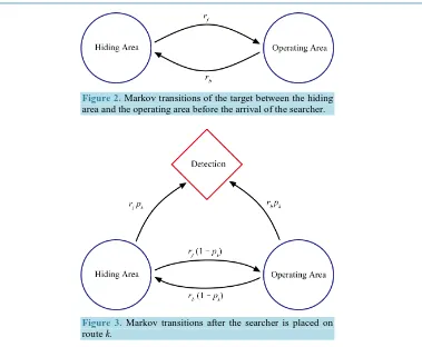
Before the arrival of the searcher, the target jumps between two Markov states with forward rate rf and back-ward rate rb, as shown inFigure 2. The steady state probabilities ( )

s h

p (hiding area) and p_o( )s (operating area) are given by

( )

s b

h

f b

f s o

f b

r p

r r

r p

r r

= +

(1)

Once the searcher arrives at route k to commence monitoring there, the diagram of Markov transitions con-tains 3 states. As shown inFigure 3, the third state is the target being detected. When the target leaves the hid-ing area, it has probability p_k of taking route k (and thus being detected). The transition rate from the hiding area to being detected is r p_f _k; the rate of going from the hiding area to the operating area (without being de-tected on the way) is r_f

(

1−p_k

)

. Similarly, the transition rate from the operating area to being detected is r p_b _k; the rate of traveling from the operating area back to the hiding area (without being detected on the way) is

(

1

)

b k

r −p .

Let p_h

( )

t and p_o

( )

t denote, respectively, the probability of being in the hiding area and that of being in the operating area at time t. The probability of the target having been detected by time t is 1−p t_h

( )

−p t_o

( )

(i.e., the probability of the third state). Notice that there is no transition from the third state back to the other two states. The time evolution of probabilities p_h

( )

t and p_o

( )

t is governed by

(

)

(

)

d

1 d

d

1 d

h

f h b k o

o

f k h b o

p

r p r p p

t p

r p p r p

t

= − + −

= − −

(2)

with initial conditions (t = 0 being the time when the searcher arrives at route k)

( )

0 b ,

( )

0 f .

h o

f b f b

r r

p p

r r r r

= =

(4)

[image:4.595.127.506.75.387.2] [image:4.595.199.431.189.379.2]

Figure 2. Markov transitions of the target between the hiding area and the operating area before the arrival of the searcher.

Figure 3. Markov transitions after the searcher is placed on route k.

operating area before the start of search. Equation (2) andFigure 3 describe the evolution of probability distri-bution after the start of search.

Both p_h

( )

t and p_o

( )

t have the general form of

( )

1exp

(

1

)

2exp

(

2

)

p t =c −λt +c −λt (4) where

( )

−λ₁ and

(

−λ₂

)

are the eigenvalues of the coefficient matrix of the linear ODE system (2). That is,

(

) (

)

(

)

(

) (

)

(

)

2 ₂

1

2 ₂

2

4 2

2

4 2

. 2

f b f b f b k k

r r r r r r p p

λ

+ + + − −

=

+ − + − −

=

(5)

The probability that the target is not detected by time t (i.e. the non-detection probability, also called the escape probability) has the same form which reads

( )

1exp

(

1

)

2exp

(

2

)

nd h o

p t = p t +p t =c −λt +c −λt (6) where the coefficients c1 and c2 are calculated below and are contained in Equation (8).

The non-detection probability is constrained by two other conditions, namely,

( )

0 1

2

0 0 0 0 0

nd

f b

nd h o h f k o b k k

f b

p

r r

p p p p r p p r p p

r r

=

′ ′ ′

− = − − = + =

+

(7)

where the second condition is derived from differential equations (2) and initial conditions (3). The two con-straints in (7) allow us to calculate the coefficients c1 and c2 in (6) explicitly. After some algebra, we find the

(5)

( )

(

1

)

(

2

)

1 1

exp exp

2 2

nd

p t = −α −λt + +α −λt (8) where the coefficient

α

is given by

(

)

(

) (

)

(

)

2 2 ₂ 4 . 4 2

f b f b k

f b f b f b k k

r r r r p

r r r r r r p p

α = + −

+ + − −

Note that

α

>0. Observe also that according to (8), the non-detection probability is a linear combination of two exponential modes: one decreases with fast rate λ₁, the other with slow rate λ₂. Since

α

>0, the slow decaying mode carries more weight, usually a lot more than the weight of the fast decaying mode.

When p_k is moderately small, we obtain the following asymptotic expansions:

(

)

(

)

( )

(

)

(

)

( )

(

)

(

( )

)

(

)

2 1 2 2 2 2 2 2 2 1 2 2 1 2 1

exp 1 exp .

f b

f b k k

f b

f b

f b k k

f b

k

nd k k

r r

r r p O p

r r

r r

r r p O p

r r

O p

p t O p t O p t

λ λ α λ λ     = + − +  ₊        = + +  ₊    = − = − + − − (9)

Therefore, when p_k is moderately small (for example, pk ≤0.1), the decay of the non-detection probability is mainly described by the slow decay rate

2 2 _{f b}

k f b r r p r r λ ≈ +

which is approximately proportional to probability p_k. Consequently, the non-detection probability simplifies approximately to

( )

exp 2 f b .

nd k

f b

r r

p t p t

r r

− 

≈ _ _

+

 

In an effort to use one quantity to characterize the decay of the non-detection probability, we compute the mean time to detection. Let T_detection denote the time to detection, which is a random variable. We calculate the mean time to detection from p_nd

( )

t given in (8):

[

]

( )

(

)

2 detection ₀ 1 2 2 1

1 1 1 1

d .

1

2 2 2 ₁

2 f b k f b f b nd

f b k

k

r r p

r r

E T p t t

r r p _p

α α λ λ ∞ − + + − + = = ⋅ + ⋅ = ⋅ −

∫

(10)

The derivative of E T

[

_detection

]

with respect to p_k is

[

]

(

)

2 2 detection 2 2 1 d 0.

d 2 ₁

1 2 f b k k f b f b

k f b k

k r r p p r r r r E T

p r r p

p

 

 ₋ ₊ 

 ₊ 

 +  _ _

= −_ _⋅ <

 

  ₋

 

 

(11)

(6)

the best choice is to place the searcher on the route that the target is most likely to journey. This is consistent with intuition. As we will see later, in the case of the target having different probabilities of taking a given route for the two travel directions, and/or in the case of more than one searcher, the straightforward intuition often fails to yield the optimal placement.

When p_k is small, it follows from (10) that the mean time to detection can be approximated by

[

detection

]

2 f b

f b k

r r

E T

r r p

+

≈ (12)

which is inversely proportional to p_k.

2.2. Case 2B: The Searcher Is Placed in the Operating Area to Scan Search the Area

Now we consider the situation where the searcher looks over only the operating area. Since the searcher is committed to searching the operating area, the target can only be detected when it is in the operating area.

Here we do not specify how the searcher conducts search over the operating area, which may include random search, parallel sweeps (mowing the lawn), spiral-in or spiral-out paths. We consider the conditional probability of the non-detection given that the target is in the operating area. We model the conditional non-detection prob-ability as a single exponential decay.

( )

(

target in operating area

)

exp

(

)

nd nd d

p t O ≡ p t = −r t (13)

where r_d is the detection rate in the operating area.

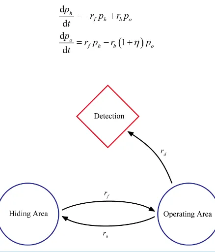
In addition to transitions between the hiding area and the operating area, there is now a new transition of the target going from the operating area to being detected. Upon the arrival of the searcher in the operating area, the Markov transitions of the target are depicted in the diagram shown inFigure 4.

For mathematical convenience, we represent the detection rate r_d as

d b

r = ⋅η r

where η:1 are the odds of being detected in a trip to the operating area. The time evolution of probabilities p_h

( )

t and p_o

( )

t is now given by

(

)

d d d

1 d

h

f h b o

o

f h b o

p

r p r p

t p

r p r p

t η

= − +

(14)

subject to initial conditions

[image:6.595.203.422.443.699.2]

(7)

( )

0 b ,

( )

0 f .

h o

f b f b

r r

p p

r r r r

= =

+ +

Proceeding exactly as for Case 2A, we can succinctly express the non-detection probability as

( )

1exp

(

1

)

2exp

(

2

)

nd

p t =c −λt +c −λt (15) where λ₁ and λ₂ are the eigenvalues of the coefficient matrix of the linear ODE system (14):

(

)

(

)

(

)

(

)

(

)

(

)

2 1 2 2

1 1 4

2

1 1 4

. 2

f b f b f b

r r r r r r

η η η

λ

η η η

λ + + + + + − = + + − + + − = (16)

The non-detection probability also satisfies two other conditions:

( )

0 1

0 0 .

nd

f b

nd o b

f b

p

r r

p p r

r r η η = ′ − = = + (17)

We solve for coefficients c₁ and c₂ in (15) from these two conditions. We obtain

( )

(

1

)

(

2

)

1 1

exp exp

2 2

nd

p t = −α −λt + +α −λt (18) where the coefficient

α

is defined by

(

)

(

)

(

)

(

)

2

2 0.

1 4

f b b b f

f b f b f b

r r r r r

r r r r r r

η α η η + + − = > + + + −

As discussed before, the non-detection probability contains two exponential modes: one decays with fast rate

1

λ , the other with slow rate λ₂. Since

α

>0, the slow decaying mode bears more weight. When

η

is mod-erately small (i.e., the probability of being detected in one trip to the operating area is mall), we arrive at the following asymptotic expansions:

(

)

(

)

( )

(

)

(

)

( )

(

)

(

( )

)

(

)

2 2 1 2 2 2 2 2 2 2 1 2 1 1

exp 1 exp .

b f b f b f b f b f b nd r

r r O

r r

r r

r r O

r r

O

p t O t O t

λ η η

α η

η λ η λ

    = + + +  ₊        = + +  ₊    = − = − + − − (19)

From the results of these asymptotic expansions, we see that when

η

is moderately small, the decay of the non-detection probability can be characterized by the slow decay rate

2 . f d f b r r r r λ ≈ +

Accordingly, the non-detection probability takes the approximate form

( )

exp f d . nd

f b

r r

p t t

r r

− 

≈ _ _

+

(8)

Again, we calculate the mean time to detection from p_nd

( )

t in (18):

[

]

( )

(

)

(

)

( )

detection ₀

1 2

1 1 1 1

d

2 2

. nd

f b b f b b

d

f b f f b f d f f b

E T p t t

r r r r r r

g r

r r r r r r r r r r

α α

λ λ

η

∞ − +

= = ⋅ + ⋅

+ +

= + = + ≡

+ +

∫

(20)

Notice that the mean time to detection contains a constant part that does not decrease with increasing detection rate r_d. This reflects the fact that no matter how fast the target can be detected in the operating area, the detection can occur only when the target moves to the operating area. The constant term

(

b

)

f f b

r

r r +r is the mean

elapsed time until the first arrival of the target in the operating area. This constant term gives the lower bound on the mean time to detection, which can be achieved when the detection rate in the operating area is much larger than other transition rates: rdmax

(

r rf,b

)

.

Combining the results of Case 2A and Case 2B, we can now determine the optimal placement of the searcher (on a particular route vs. in the operating area ) in order to attain the minimum mean time to detection of the target. We introduce the probability and identify of the route that is most likely to be travelled by the target:

( )

max max j

j

p = p

( )

max arg max j . j

k = p

We compare the mean times to detection in the two cases

(

)

(

)

max 2

max

2 1

vs. .

1 2

f b

f b

f b f b b

f b f d f f b

r r p

r r

r r r r r

r r p _p r r r r r

− +

+ +

⋅ +

+ −

If the former is smaller, we place the searcher on route k_max, the route with the highest probability of being tra-veled by the target; if the later is smaller, we place the searcher in the operating area to scan search the area. Note that when the probability of taking a given route is the same for the two travel directions, the minimum mean time to detection among all routes is the one corresponding to the route most likely to be traveled by the target. This is consistent with intuition. This intuitive strategy, however, breaks down when the probability of taking a given route has different values for the two travel directions. That situation is discussed in the next section.

3. A Target Having Different Probabilities of Taking a Given Route for the Two

Travel Directions

In this section, we consider the target which behaves the same as in Section 2 except that the probability of tak-ing route k may have different values for the forward travel (from the hiding area to the operating area) and the backward travel (from the operating area to the hiding area). We use p_k and q_k to denote, respectively, the probabilities of taking route k in the two opposite travel directions. More specifically,

• On its travel from the hiding area to the operating area, the target takes route k with probability p_k. • On its travel from the operating area back to the hiding area, the target chooses route k with probability q_k.

We study the performance of placing the searcher on a route, which is analogous to Case 2A. Note that re-gardless of the target’s behavior in selecting which route to take, the results of Case 2B apply directly here, which is affected only by how frequently the target visits the operating area and how fast the target is detected while in the operating area.

Case 3A: The Searcher Is Placed on Route

k

(9)

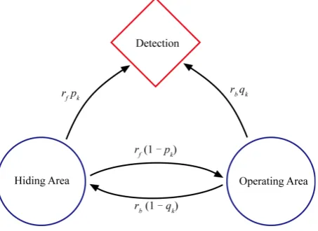
Figure 5. Markov transitions after the searcher is placed on route k in Case 3A where the probability of taking route k is

pk for the forward travel and qk for the backward travel.

being detected). The transition rate from the hiding area to being detected is r p_f _k; the rate of going from the hiding area to the operating area (without being detected on the way) is r_f

(

1−p_k

)

. Likewise, on the target’s returning trip to the hiding area, the transition rate from the operating area to being detected is r q_b _k; the rate of traveling from the operating area back to the hiding area (without being detected on the way) is r_b

(

1−q_k

)

.

The time evolution of probabilities p_h

( )

t and p_o

( )

t follows a set of ODEs:

(

)

(

)

d

1 d

d

1 d

h

f h b k o

o

f k h b o

p

r p r q p

t p

r p p r p

t

= − + −

= − −

(21)

with initial conditions

( )

0 b ,

( )

0 f .

h o

f b f b

r r

p p

r r r r

= =

+ +

The non-detection probability is of the form

( )

1exp

(

1

)

2exp

(

2

)

nd

p t =c −λt +c −λt (22) where λ₁ and λ₂ are the eigenvalues of the coefficient matrix of the linear ODE system (21)

(

) (

)

2

(

)

1

4

2

f b f b f b k k k k

r r r r r r p q p q

λ

= + + + − + −

(

) (

)

2

(

)

2

4

. 2

r r r r r r p q p q

λ

= + − + − + −

The non-detection probability needs to meet two more conditions:

( )

(

)

0 1

0 0 0 .

nd

f b

nd h f k o b k k k

f b

p

r r

p p r p p r q p q

r r

=

′

− = + = +

+

With the help of these two constraints, we can determine the coefficients c₁ and c₂. We write out the non- detection probability as

( )

(

1

)

(

2

)

1 1

exp exp

2 2

nd

[image:9.595.202.429.87.252.2]

(10)

with the coefficient

α

satisfying

(

)

(

)

(

) (

)

(

)

2 2 2 0. 4

f b f b k k

r r r r p q

α = + − + >

+ + − + −

As in the earlier discussion, the non-detection probability is a linear combination of two exponential modes: one decreases with fast rate λ₁ while the other with slow rate λ₂. The fact that

α

is positive suggests that the slow decaying component weighs more than the fast decaying one.

When both p_k and q_k are moderately small, we carry out the asymptotic analysis to obtain

(

)

(

)

(

)

(

)

(

)

(

)

(

)

(

)

(

)

( )

(

)

(

)

(

)

(

)

2 2 1 2 2 2 2 2 2 2

2 2 2 2

1 2

1

exp 1 exp .

f b

f b k k k k

f b

f b

f b k k k k

f b

k k

nd k k k k

r r

r r p q O p q

r r

r r

r r p q O p q

r r

O p q

p t O p q t O p q t

λ λ α λ λ     = + − + + +  ₊        = + + + +  ₊    = − + = + − + − + − (24)

It therefore follows that when p_k and q_k are moderately small (for example, pk ≤0.1 and qk≤0.1), the decay of the non-detection probability is dominated by the slow decay rate

(

)

2 f b k k f b r r p q r r

λ ≈ +

+

which is approximately proportional to probability

(

p_k+q_k

)

. Furthermore, the non-detection probability is well approximated by

( )

exp f b

(

)

.

nd k k

f b

r r

p t p q t

r r

 − 

≈ _ + _

+

 

Next we find the mean time to detection. Using the formula (23), we compute the mean time to detection:

[

]

(

)

(

)

(

)

2 detection 1 2 1

1 1 1 1

, . 2 2 f b k k f b f b k k f b k k k k

r r

p q

r r

E T h p q

r r p q p q

α

λ

− + + + − + = ⋅ + ⋅ = ⋅ ≡

+ − (25)

The most important thing to notice about this result is that the mean time to detection is not just a function of

(

pk+qk

)

, the sum of probabilities of taking route k in the two travel directions. Consequently, the optimal route is not necessarily the one that has the largest value of

(

p_k+q_k

)

. To illustrate this point, we consider a simple and interesting example in the following.

An Example: Let us consider a target traveling between the hiding area and the operating area. The transition rates and the probabilities of taking individual routes in each travel direction are listed below.

0.1, 1

f b

r = r =

(

p p p p1, 2, 3, 4

) (

= 0.47, 0.35, 0.13, 0.05

)

(

q q q q1, 2, 3, 4

) (

= 0.15, 0.3, 0.0, 0.55

)

The small value for r_f corresponds to the fact that the target stays in the hiding area for most time. If we compute the values of p_k+q_k, we have

1 1 0.62, 2 2 0.65, 3 3 0.13, 4 4 0.6.

p +q = p +q = p +q = p +q =

(11)

k k

p +q ; the second candidate for the optimal route seems to be k=1, which leads to the second largest value of p_k+q_k. However, to select the optimal route for placing the searcher, we appeal to (25) and calculate the mean time to detection for each route:

(

)

detectionroute 1 1, 1 18.99

E T_  =_ h p q =

(

)

E T_  =_ h p q =

(

)

E T_  =_ h p q =

(

)

E T_  =_ h p q =

It is clear that route 4 has the smallest mean time to detection, and thus, is the optimal route for placing the searcher. This example highlights that when the probability of taking a given route has different values for the two travel directions, the optimal placement of the searcher is not the one suggested by straightforward intuition.

4. A Moving Target and Two Searchers

We study the effect of two searchers where each searcher acts and detects independently. We assume the same setup for the target as in Section 3. The difference here is that there are two cookie-cutter searchers deployed in search for the target. We consider several options of placing the two cookie-cutter searchers.

4.1. Case 4A: Both Searchers Are Placed on Routes: One on Route

k

and the Other on

Route

j

Since we assume that one searcher is capable of covering the full width of a route, there is absolutely no benefit for placing more than one searchers on any one route. Thus, the two searchers are to be placed on two different routes. In this case, the mathematical formulation is exactly the same as in Case 3A in Section 3 except that probability p_k in Section 3 is now replaced with the effective probability p_k+p_j; and in place of q_k in Case 3A we have q_k+q_j. We introduce two short notations that will be convenient throughout this section:

, .

k j k j

p≡ p +p q≡q +q (26) Then, the non-detection probability is given by

( )

(

1

)

(

2

)

1 1

exp exp

2 2

nd

p t = −α −λt + +α −λt (27)

where eigenvalues λ₁ and λ₂, and coefficient

α

are

(

) (

)

2

(

)

1

4 (

2

f b f b f b

r r r r r r p q pq

λ

= + + + − + −

(

) (

)

2

(

)

2

4

2

f b f b f b

r r r r r r p q pq

λ

= + − + − + −

(

)

(

)

(

) (

)

(

)

2

0 4

f b f b

f b f b f b

r r r r p q

r r r r r r p q pq

α = + − + >

+ + − + −

Recalling (25) obtained in Case 3A of Section 3, one finds the mean time to detection in the form

[

detection

]

(

,

)

E T =h p q (28)

(12)

(

)

(

)

(

)

2

1

,

f b

f b f b

f b

r r

p q

r r

h p q

r r p q pq

− +

+ +

≡ ⋅

+ − (29) The optimal routes for placing the two searchers are selected by minimizing the mean time to detection:

( )

_{( )}

(

)

,

, arg min _k _j, _k _j , .

k j

k j = h p +p q +q k≠ j

It is attempting to simplify the selection process by using the optimal route for a single searcher plus the second optimal route for a single searcher. The example below demonstrates that this intuitive approach does not necessarily give us the optimal routes for placing the two searchers.

An example: We consider a target traveling between the hiding area and the operating area over 5 routes. The transition rates and the probabilities of taking route k in the two travel directions are given below for the target

0.1, 1

f b

r = r =

(

p p p p p1, 2, 3, 4, 5

) (

= 0.45, 0.0, 0.25, 0.25, 0.05

)

(

q q q q q1, 2, 3, 4, 5

) (

= 0.0, 0.46, 0.25, 0.25, 0.04 .

)

When only a single searcher is present, the mean times to detection for individual routes are calculated from (25)

(

)

E T_  =_ h p q =

(

)

E T_  =_ h p q =

(

)

E T_  =_ h p q =

(

)

E T_  =_ h p q =

(

)

E T_  =_ h p q =

The optimal route and the second optimal route for placing a single searcher are, respectively, route 2 and route 1. It seems reasonable to conclude that in the case of two searchers, the optimal routes for placing the two searchers are routes 2 and 1. However, this is not true. When the two searchers are placed respectively on routes 1 and 2, the mean time to detection is then obtained from (28) as

( )

(

)

detectionroute 1,2 1 2, 1 2 14.47.

E T_  =_ h p +p q +q =

In comparison, when the two searchers are placed respectively on routes 1 and 3, the mean time to detection be-comes

( )

(

)

detectionroute 1,3 1 3, 1 3 13.81

E T_  =_ h p +p q +q =

which is still not yet the optimal. It turns out that the smallest mean time to detection among all possible pairs of routes is achieved by placing the two searchers respectively on routes 3 and 4:

( )

(

)

detectionroute 3,4 3 4, 3 4 13.46.

E T_  =_ h p +p q +q =

In this example, the optimal pair of routes for placing the two searchers are routes 3 and 4, not the collection of optimal and second optimal routes for a single searcher.

(13)

operating area is patrolled by two searchers.

Based on the results in Case 2B of Section 2, the mean time to detection can be written as

[

detection

]

( )

2d

E T =g r (30) where function g

( )

β is defined in (20). That is,

( )

f b

₍

b

₎

.

f f f b

r r r

g

r r r r

β

β +

≡ +

+

4.3. Case 4C: One Searcher Is Placed on Route

k

and the Other in the Operating Area

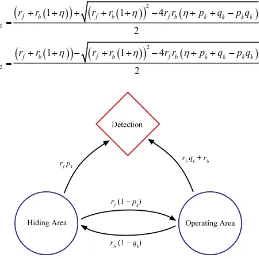
The last mathematical formulation is for the case where one searcher is put on a pathway while the other scans the operating area. After the arrival of one searcher at route k and the other in the operating area, the target evolves stochastically according to the Markov process shown inFigure 6.

For mathematical convenience, we express the detection rate r_d in the operating area as r_d= ⋅η r_b. The go-verning equations for the time evolution of probabilities p_h

( )

t and p_o

( )

t consist of

(

)

(

)

(

)

d

1 d

d

1 1 .

d

h

f h b k o

o

f k h b o

p

r p r q p

t p

r p p r p

t η

= − + −

= − − +

(31)

These probability functions satisfy the initial conditions

( )

0 b ,

( )

0 f .

h o

f b f b

r r

p p

r r r r

= =

+ +

Once again, one finds that the non-detection probability has the form

( )

1exp

(

1

)

2exp

(

2

)

nd

p t =c −λt +c −λt (32) where λ₁ and λ₂ correspond to the two eigenvalues of the coefficient matrix of the linear ODE system (31):

(

)

(

)

(

)

2

(

)

1

1 1 4

2

r r

η

r r

η

r r

η

p q p q

λ

= + + + + + − + + −

(

)

(

)

(

)

2

(

)

2

1 1 4

2

r r

η

r r

η

r r

η

p q p q

λ

= + + − + + − + + −

[image:13.595.185.444.439.698.2]

(14)

The coefficients c1 and c2 can be derived by imposing two constraints on the non-detection probability:

( )

( ) (

)

(

)

0 1

0 0 0 .

nd

f b

nd h f k o b k k k

f b

p

r r

p p r p p r q p q

r r

η η

=

′

− = + + = + +

+

From these two constraints, one derives that the non-detection probability is given by

( )

(

1

)

(

2

)

1 1

exp exp

2 2

nd

p t = −α −λt + +α −λt (33) where coefficient

α

is

(

)

(

)

(

)

(

)

(

)

(

)

2

.

1 4

f b b b f f b k k

r r r r r r r p q

η α

η η

+ + − − +

=

+ + + − + + −

The mean time to detection is calculated from the non-detection probability p_nd

( )

t given in (33). The result-ing mean time to detection is equal to:

[

]

(

)

(

)

(

)

(

)

(

)

(

)

(

)

(

)

detection

1 2

2

2 2

1 1 1 1

2 2

1

, , .

f b b

k k

f b f b

f b

f b k k k k

f b b

d k k

f b f b

f b

f d b k k k k

d k k

E T

r r r

p q

r r r r

r r

r r p q p q

r r r

r p q

r r r r

r r

r r r p q p q

f r p q

α α

λ λ

η

− +

= ⋅ + ⋅

+ − +

+ +

 + 

=_ _⋅

+ + −

 

+ − +

+ +

 + 

=_ _⋅

+ + −

 

≡

(34)

This result lies at the heart of everything else that is going on and it includes all of these as special cases. In particular, function h p q

(

,

)

and function g r

( )

_d can be expressed in terms of function f r p q

(

d, k, k

)

as:

(

,

)

(

0, ,

)

h p q = f p q

( )

_d

(

_d, 0, 0 .

)

g r = f r

We are now ready to summarize what we have found so far.

4.4. Optimal Placement of Two Searchers

When the two searchers are placed on two routes k and j (one searcher on each route), the shortest mean time to detection is given by

( ),

(

)

min 0, _k _j, _k _j , . k j f p +p q +q k≠ j

When one searcher is placed on route k and the second searcher is placed in the operating area, the smallest mean time to detection is similarly defined by

(

)

min d, k, k .

k f r p q

When both searchers are placed in the operating area, the mean time to detection is

(

2 , 0, 0 ._d

)

f r

(15)

( ),

(

)

(

) (

)

min min 0, _k _j, _k _j , min _d, _k, _k , 2 , 0, 0_d

k j f p p q q k f r p q f r

 ₊ ₊ 

 

 

where function f

(

β, ,p q

)

is defined by

(

)

(

)

(

)

(

)

(

)

2 2

1

, , .

f b b

f b f b

f b

r r r

p q

r r r r

r r

f p q

r r p q pq

β β

β

+ − +

+ +

 + 

≡_ _⋅

+ + −

  (35)

5. Three or More Searchers

We now turn to the case where three cookie-cutter searchers are deployed in the search for the target. Probabil-istic independence is assumed for each searcher. Suppose the target behaves exactly the same as described in Sections 3 and 4. We apply function f

(

β, ,p q

)

to calculate the optimal placement of the three searchers.

When all three searchers are placed on three routes (one searcher on each route), the shortest mean time to detection is found to be

(mink j i, ,)f

(

0,pk+pj+p qi, k +qj+qi

)

.

Similarly, when two searchers are placed on two routes (one searcher on each route) and the third searcher is placed in the operating area, the shortest mean time to detection is

( ),

(

)

min _d, _k _j, _k _j . k j f r p +p q +q

When one searcher is placed on route k and the two other searchers are placed in the operating area, the smallest mean time to detection is equal to

(

)

min 2 ,d k, k .

k f r p q

Finally, when all three searchers are placed in the operating area, it follows that the mean time to detection is

(

3 , 0, 0 ._d

)

f r

We conclude that the overall minimum mean time to detection over these options can be computed by compar-ing the results in these cases

( , ,)

(

)

( ),

(

)

(

) (

)

min min 0, _k _j _i, _k _j _i , min _d, _k _j, _k _j , min 2 ,_d _k, _k , 3 , 0, 0_d .

k j i f p p p q q q k j f r p p q q k f r p q f r

 ₊ ₊ ₊ ₊ ₊ ₊ 

 

 

It is also evident that this method can be extended to finding the optimal placement for any number of searchers.

6. Conclusions

This paper presented a mathematical approach to investigate the search problem of detecting a mobile target that travels between a hiding area and an operating area over a collection of fixed pathways in the presence of single or multiple searchers with cookie-cutter sensors. Both the dwell time of the target in the hiding area and the dwell time of the target in the operating area were assumed to be exponentially distributed and were modeled mathematically by Markov transition rates. The travel time of the target on a pathway was assumed to be short in comparison with the dwell times in the hiding area and the operating area. The target took a route to and from the operating area based on a probability distribution. Under these assumptions, a mathematical formulation was developed and solved analytically.

The main results can be summarized as follows.

1) When only one searcher is present, one can compute the mean time to detection, respectively, when the searcher is placed on route k or when the search is placed in the operating area. By comparing the mean times to detection, we can decide whether to put the searcher on a certain route or in the operating area.

(16)

searchers.

It was discovered that in many cases the optimal search design was not necessarily the one indicated by straightforward intuition.

There are a few possible future research directions. For example, extending current study to include time- dependent transition rates and detection rates would provide a more sophisticated modeling. Multiple targets could also be considered in the future studies.

Acknowledgements and Disclaimer

Hong Zhou would like to thank Naval Postgraduate School Center for Multi-INT Studies for supporting this work. Special thanks go to Professor Jim Scrofani and Deborah Shifflett. The views expressed in this document are those of the authors and do not reflect the official policy or position of the Department of Defense or the U.S. Government.

References

[1] Koopman, B.O. (1999) Search and Screening: General Principles with Historical Applications. The Military Opera-tions Research Society, Inc., Alexandria.

[2] Stone, L.D. (1989) Theory of Optimal Search. 2nd Edition, Operations Research Society of America, Arlington.

[3] Wagner, D.H., Mylander, W.C. and Sanders, T.J. (1999) Naval Operations Analysis. 3rd Edition, Naval Institute Press, Annapolis.

[4] Washburn, A. (2014) Search and Detection. 5th Edition, Create Space Independent Publishing Platforms.

[5] Chung, H., Polak, E., Royset, J.O. and Sastry, S. (2011) On the Optimal Detection of an Underwater Intruder in a Channel Using Unmanned Underwater Vehicles. Naval Research Logistics, 58, 804-820.

http://dx.doi.org/10.1002/nav.20487

[6] Chung, T.H., Hollinger, G.A. and Isler, V. (2011) Search and Pursuit-Evasion in Mobile Robotics. Autonomous Robots,

31, 299-316. http://dx.doi.org/10.1007/s10514-011-9241-4

[7] Chung, T.H. and Silvestrini, R.T. (2014) Modeling and Analysis of Exhaustive Probabilistic Search. Naval Research Logistics, 61, 164-178. http://dx.doi.org/10.1002/nav.21574

[8] Kress, M. and Royset, J.O. (2008) Aerial Search Optimization Model (ASOM) for UAVs in Special Operations. Mili-tary Operations Research, 13, 23-33. http://dx.doi.org/10.5711/morj.13.1.23

[9] Wang, H. and Zhou, H. (2015) Computational Studies on Detecting a Diffusing Target in a Square Region by a Statio-nary or Moving Searcher. American Journal of Operations Research, 5, 47-68.