Munich Personal RePEc Archive
Evidence of preference construction in a
comparison of variants of the standard
gamble method
Brazier, J and Dolan, P
The University of Sheffield
December 2005
Online at
https://mpra.ub.uni-muenchen.de/29760/
HEDS Discussion Paper 05/04
Disclaimer:
This is a Discussion Paper produced and published by the Health Economics
and Decision Science (HEDS) Section at the School of Health and Related
Research (ScHARR), University of Sheffield. HEDS Discussion Papers are
intended to provide information and encourage discussion on a topic in
advance of formal publication. They represent only the views of the authors,
and do not necessarily reflect the views or approval of the sponsors.
White Rose Repository URL for this paper:
http://eprints.whiterose.ac.uk/10936/
Once a version of Discussion Paper content is published in a peer-reviewed
journal, this typically supersedes the Discussion Paper and readers are invited
to cite the published version in preference to the original version.
Published paper
None.
The University of Sheffield
ScHARR
School of Health and Related Research
Health Economics and Decision Science
Discussion Paper Series
December 2005 Ref: 05/4
Evidence of preference construction in a comparison of
variants of the standard gamble method
John Brazier and Paul Dolan
Corresponding Author: John Brazier
Health Economics and Decision Science School of Health and Related Research University of Sheffield
Regent Court, Sheffield, UK S1 4DA
Email: [email protected]
ABSTRACT
An increasingly important debate has emerged around the extent to which techniques
such as the standard gamble, which is used, amongst other things, to value health states,
actually serve to construct respondent’s preferences rather than simply elicit them.
According to standard theory, the variant used should have no bearing on the numbers
elicited from respondents i.e. procedural invariance should hold. This study addresses
this debate by comparing two variants of standard gamble in the valuation of health
states. It was a mixed methods study that combines a quantitative comparison with the
probing of respondents in order to ascertain possible reasons for the differences that
emerged. Significant differences were found between variants and, furthermore, there
was evidence of an ordering effect. Respondents’ responses to probing suggested that
they were influenced by the method of elicitation.
1. INTRODUCTION
The Standard Gamble (SG) method asks respondents to compare a certain outcome with
a risky gamble, which will result in a better outcome if the gamble pays off and a worse
outcome if it does not. The method can be used to value anything from wealth to
health. In valuing health, an individual is presented with an intermediate health state,
hi, and asked to find a point of indifference between this state with certainty and a
gamble with a p* chance of a better outcome (usually full health) and a 1-p* chance of a
worse outcome (often this is death). If full health and death are set to one and zero,
respectively, then, according to the axioms of expected utility theory (EUT), hi = p.
The SG response therefore yields a cardinal index measuring an individual’s utility
under uncertainty (Von Neumann and Morgenstern, 1944). This index is unique up to a
positive linear transformation and therefore provides an interval scale. The axiomatic
basis of SG in the classical theory of decision-making under uncertainty seems highly
relevant to medical decisions, and this has led to it being regarded by many health
economists as a ‘gold standard’ amongst valuation techniques in health care (Mehrez
and Gafni, 1993; Drummond et al., 1997).
However, there is a considerable body of evidence in relation to prospects involving
wealth, and an increasing amount of evidence in the field of health, which raise serious
doubts about the descriptive validity of the restrictions imposed by EUT (Schoemaker,
1982; Loomes, 1993; Oliver, 2003). Notwithstanding this, the SG has become one of
the main techniques for putting the ’Q’ into the Quality Adjusted Life Year (QALY),
which combines health state values and duration into a single index number (Dolan,
years, a number of different variants of the SG have been developed and, if people’s
preferences are not as well constructed as standard economic theory would suggest, it is
not at all clear that different variants will generate the same values.
A criticism of the current methods for eliciting preferences using techniques such as SG
is that the tasks are cognitively complex, with respondents being asked to consider
variations in numerous attributes simultaneously across choices involving at least three
scenarios, with the added complexity of probabilistic information. Evidence from
psychology would suggest that respondents faced with such complex problems would
tend to adopt simple heuristic strategies (Lloyd, 2003). This would be particularly true
where the respondents have little time to consider their real underlying values. A
worrying concern that has emerged from the psychology literature is that techniques
such as SG may actually construct respondent’s preferences in some way rather than
simply eliciting them (Slovic, 1995). This would suggest that the precise wording of the
SG question might influence the answers given.
Over the last 30 or so years different variants of the SG have been developed in order to
assist the respondent as much as possible and promote standardisation through the use
of different elicitation procedures, the use of visual aids and different methods of
administration. While such development of methods might be regarded as laudable, it
does raise the question of whether different variants result in systematic differences.
EUT does not suggest one variant of SG should be preferred to another and, indeed, the
precise framing of the question should not influence the result as, according to EUT,
people have well-constructed preferences. If elicitation techniques do construct
respondents will be influenced by factors extraneous to the health states being valued,
such as the framing of the question.
This study compares two variants of the more widely used variants of SG in the health
and transport economic literatures. The study compared the ‘ping pong’ method, based
on a method developed by Furlong and others (1990) and the ‘titration’ method, first
used in a study to value injury states by Jones-Lee and colleagues (1993). The aim was
to test the hypothesis that these techniques elicit preferences and therefore there should
be no systematic difference between them. The study was specifically concerned with
the valuation of a set of health states. It was a mixed methods study that combines a
quantitative comparison with the probing of respondents in order to ascertain possible
reasons for any apparent inconsistencies in health state values from using one variant
compared to the other.
2. METHODS
2.1 Participants
The participants were recruited from staff and students at the University of Sheffield
Medical School. No payment was offered to the participants in this study. A research
assistant was given a list of names of staff and students at the institution and then
randomly drew names from the lists. Once recruited respondents were randomised
between each of two groups who completed different questionnaires. The same
2.2 The Variants
2.2.1 The ‘ping pong’ variant
The ping pong variant (PPV) is administered by interview and employs a visual aid
where the probabilities are displayed on a board, both numerically and in the form of a
pie chart. A key feature of this variant is that the probability of success is presented in a
‘’ping pong’ fashion that oscillates up and down the scale. The respondent is asked to
choose between the ill-health state for certain compared to the uncertain prospect of a
risky treatment, where the outcomes are full health and some worse outcome.
The first question asked respondents to consider this choice where the probability of
success is set at 1.0. This is a test question is to ensure the respondent understands the
health state classification. Should they choose the certain intermediate state over being
in full health for certain, they are asked the reason for this. Such a choice is rarely made.
The probability of the best outcome is then changed to 0.1. Should the respondent
choose the uncertain treatment, then the assumed indifference value is 0.05. If they
choose the certain ill health state then the probability of success is increased to 0.9.
Should the respondent then choose the certain prospect, he/she would be asked to
explicitly consider the probability of the best outcome being 0.95. Where the respondent
continues to choose the certain prospect, then the interpolated value for indifference is
0.975 and where the respondent chooses the uncertain prospect, the value is 0.925.
A respondent who chooses the uncertain prospect at a probability of 0.9 would be asked
would then result in the respondent being asked to consider a probability of 0.8. This
procedure continues in a ‘ping pong’ fashion until the respondent’s point of indifference
is revealed. The probabilities are presented in units of 0.1 except for 0.95, which
generate values on a scale from 1.0 to zero in intervals of 0.05 (except for 0.975).
The board is designed to ensure each interview is standardised in order to minimise the
risk of interviewer variation. The board and pie chart are also designed to help the
respondents understand the notion of probability. The developers have tried and tested
the procedure over many years and it has become widely used in health economics,
including the valuations of two of the leading generic instruments, the Health Utility
Indices-3 and the SF-6D (Feeney et al, 2002; Brazier et al, 2002).
2.2.2 The titration variant
For the titration variant (TV), the chances of success are listed from 100 in 100 down to
0 in 100 in intervals of 5, which generates a scale from 1.0 to zero in intervals of 0.025.
It is usually self-completed following instruction from the interviewer. Respondents are
asked to place a tick against all the probabilities of success at which they are confident
they would choose the treatment and a cross against all the values where they would
reject the treatment. They are then asked to indicate the chances of success at which
they would find it most difficult to choose. Where this region covers more than one
probability value, then a mid-point is taken to be the indifference value. This version of
SG has been found to produce more consistent and reliable data than an interview based
In summary, as their names suggest the variants differ in terms of their procedure for
finding the indifference probability value. However, they also differ in the way they are
administered (i.e the PPV is interviewer administered and TV is seclf-completed witht e
interviewer in attendance) and in the use of props (i.e. PPV has props, whereas the TV
does not). Both instruments generate indices on the same zero to one scale, with PPV
generating a distribution of scores with 0.05 intervals, except at the top end where there
is an additional value of 0.975 (due to respondents being offered 0.95), and TV
generates intervals of 0.025. It is possible for differences within individuals of 0.05 to
arise due to ‘rounding’.
2.3 The interviews
In both groups respondents were asked to complete the SF-6D, a health state
classification developed from the SF-36. The SF-6D describes health across six
multi-level dimensions: physical functioning, role limitations, social functioning, pain, mental
health and vitality (Brazier et al, 2002). Health states are defined by the SF-6D by
taking one level from each dimension, an example of which is shown on Figure 1.
[INSERT FIGURE 1 HERE]
Respondents were asked rank eight SF-6D health states, and then rate them using a
visual analogue scale, where the endpoints are the best and worst imaginable health
state. The eight health states were full health, the worst state defined by the SF-6D and
states were selected to represent a range of states from very mild through to severe
states defined by the SF-6D. The six intermediate states have been selected in pairs,
where each pair of states differed in a single level of one dimension.
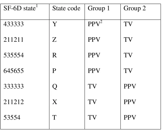
[INSERT TABLE 1 HERE]
This closeness of the three pairs has been designed to examine consistency across
methods. For each pair of health states, one state can be regarded as logically better or
worse than the other. One state will dominate over another where is better on one
dimension level and no worse across the other dimensions. The health states were
selected in adjacent pairs in order to scrutinise the consistency of respondent’s
valuations that differ by one level in one dimension. A health state is represented on
Table 1 by 6 digits, where each digit indicates the level for each of the six different
dimensions. One pair is health state Z (211211) and state X (211212) and the codes
indicate that state Z is better in vitality than state X and no worse on any other
dimension and so should dominate it. For the other pairs the logical ordering is Q>Y
and T>R.
Respondents were asked to also value each of the six intermediate states and the worst
(or ‘pits’ state), P, by SG. Each group valued these states in the same order. Group 1
valued the first four states using PPV (including P) and then valued the remaining three
states valued by the TV variant (Table 1). Group two valued the first four states by TV
and the other three by PPV. All respondents were interviewed by the same research
assistant who had been trained in the two methods by the authors in the use of the
The six intermediate states were valued in gambles containing the best state defined by
the SF-6D and the worst state P as the uncertain outcomes. P was then valued against
full health and death.
At the end of the interview, respondents were asked their gender, age, employment and
educational status. They were then asked to comment on the questionnaire. Where
inconsistencies occurred in their valuations of states between the three pairs of states (Z
and X, Q and Y and T and R), respondents were asked to comment on the reasons for
them. Respondents were then asked how difficult they found each variant and how
well they understood the tasks using five point likert scales.
2.4 Analysis
The results reported in this paper focus on mean health state values by variant and
respondent Group. The significance of any differences found is tested at the 5% level
using the t-test. An important check on the extent to which respondents were able to
understand the valuation tasks was to examine the logical consistency of their responses
and this has been presented in terms of strict inconsistency, which is where there is a
reversal of rank from the logical ordering of the states. Differences in the answering the
questions on degree of difficulty and understanding were tested using the Wilcoxon
3. RESULTS
A total of 58 respondents were recruited from staff in the Medical Faculty at the
University of Sheffield. There were 28 respondents in Group 1 and 30 in Group 2. The
groups were comparable in terms of gender (9 males in group 1 versus 10 males in
group 2), age (38 vs. 36) and own health status according to a VAS rating (0.88 vs.
0.88). The two groups ranked the states in a very similar order and their VAS ratings of
the states were virtually the same with no significant differences (Table 2).
[INSERT TABLE 2 HERE]
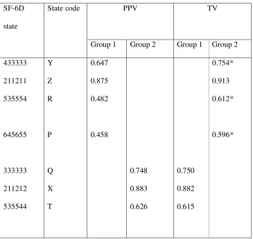
The mean SG health state values are shown on Table 3 by variant and group. Mean
health state values generated by the TV variant are higher than those produced by the
PPV for health states Y, Z, R and P. The differences are .107, .038, .130 and .138
respectively and all are significant except Z. For states X, Q and T there are little or no
difference between the variants.
[INSERT TABLE 3]
The differences between the variants can also been seen in the number of times
respondents choose to take no risk (i.e. p=1.0), which was 25 for TV compared to 6 for
PPV out of a possible 203 occasions for each variant across the 58 respondents.
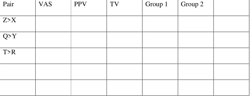
In terms of consistency with the logical ordering across the three pairs of states (i.e.
Z>X, Q>Y, T>R), the pattern is mixed (Table 4). The mean VAS values are consistent
variant and between variant. Strict inconsistencies arises between Z and X within the
PPV variant and between Q and Y for TV. Between variant inconsistencies was
measured within group, since each group valued the same states but used different
variants. Therefore, Group 1 was inconsistent between Z (PPV) and X (TV) and Group
2 between Q (TV) and Y (PPV).
[INSERT TABLE 4 HERE]
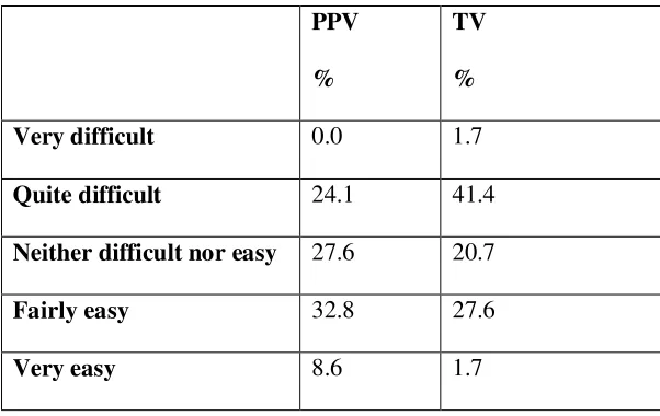
In terms of difficulty, most respondents found the two variants between quite difficult
through to fairly easy (Table 5). Only one person found either technique very difficult.
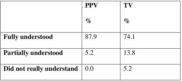
However, the responses indicate a significant difference in favour of the PPV. In terms
of understanding the tasks, most respondents said they fully understood the tasks for
both the variants, but again there was again a small and significant difference in favour
of PPV (Table 6).
[INSERT TABLES 5 AND 6 HERE]
Respondents with inconsistent responses were asked to comment on why they thought
the difference arose. Twenty-four people responded to this question. The most
common reason given by respondents was confusion, including finding it ‘hard to
remember’ and ‘forgot’. A number of respondents thought the tasks might have been
responsible for the difference: the ‘board leads to more risk taking – more attractive’
and the PPV ‘yo’s, yo’s you around whereas TV makes you more cautious’. Some
Finally, respondents were asked whether there were any other differences between the
variants. The most common comment (n=16) was that they found using the board
easier and many liked the visual aid provided by the PPV (n=7). A smaller number of
respondents (n=4) commented that they found the PPV props confusing and offering
only a limited number of choices (n=2).
4. DISCUSSION
The SG is based firmly on the axioms of EUT and is widely used to value health states.
According to EUT is does not matter which variant of the method is used as people have
well-constructed preferences. But the evidence from this study does not support the
hypothesis that these two variants of SG produce the same answers. Overall, it would
seem that TV tends to generate higher health state values than PPV. For four of the
states the differences were in excess of the 0.03 suggested in the health economics
literature as being potentially important (O’Brien and Drummond, 1996) and for three
states exceeded 0.1. This could have a potentially important impact on results of the
final incremental cost per QALY of an intervention. However, this result was only
clear for four out of the seven states. For three states the differences were very small
and two of these were in the opposite direction. These mixed results suggest that there
may be more than one reason for the differences found.
The four states where TV exceeded PPV were also the first states valued by each group.
This suggests that the valuation of the second set of states may have been contaminated
in some way by the valuation of the first four states. The first four states represent a
‘pure’ comparison of variants whereas the other three states have been altered by the
three states were lower than would otherwise be the case since they were ‘dragged
down’ by the respondent’s memory of the valuation of the first four states by PPV. For
Group 2, the PPV valuation of the last three states were ‘dragged up’ by the TV
valuation of the first four states. The net effect of this contamination from the ordering
of the variants is to offset the impact of the variant effect.
The anchoring and adjustment heuristic described by Tversky and Kahneman (1974)
results in preferences that are influenced by the provision of different anchors and is
caused by respondents making insufficient adjustment away from the starting point.
Such starting point biases have previously been found in a range of contexts, including
assessments of probabilistic information (Kahneman, 1992), contingent valuation
questions (Boyle et al, 1997) and distributional questions (Dolan and Robinson, 2002).
It seems that they may also have influenced the results reported here.
The combination of variant and ordering effects helps to explain some of the anomalies
in the inconsistency results. Within Group, the variant effect explain the inconsistencies
of X>Z and Y>Q (see Table 4). In group 1, state X was valued by TV and Z by PPV
and in group 2 state Y was valued by TV and Q by PPV. Of course the differences are
quite modest because the ordering effect has substantially negated the variant effect.
Within variant, the inconsistencies of X>Z and Y>Q have arisen from ordering effects.
States X and Q occur in the second half of the interview where the valuation has been
contaminated by the previously used variant, for example the PPV values of X increased
The fact that TV values exceed PPV values could be explained by anchoring since TV
starts eliciting preferences at the upper end of the scale, whereas the PPV iterates
respondents between the upper and lower ends, thereby reducing any anchor point bias.
An alternative view, expressed by some respondents, was that the ping pong procedure
actually confuses people and encourages them to take risk. This is supported by the
finding that that a significantly lower proportion respondents chose a probability of
success of 1.0 with PPV compared to TV.
This may arise from respondents completing PPV being encouraged to gamble at the
start of the task by the question that asks them to decide between a 100% chance of
ending up in full health or the chronic state for certain. People realise that the ill health
state is worse than full health and therefore say they would prefer full health, but then
they thrown to the other end of the scale with a 10% chance of hull health versus the
certain state. Whereas they regarded the chronic state as only slightly worse than full
health and may have preferred to take a much smaller risk than is being offered. By
contrast, the TV allows people to concentrate at the upper end and may decide on
further consideration to choose 1.0 out of the risks being made available or the next one
down. However, TV can be criticised for anchoring values at the top end.
In more general terms, this study supports a view that people’s preferences for
intangible things like health are quite labile and can be influenced by the problem
structure, question format or other aspects of the assessment process rather than simply
the content of the thing being valued. Previous studies have by Dolan et al (1996) and
Lenert et al (1998) have found that the variant of SG and TTO can influence the result.
influence the result through the ordering in which respondents undertake the tasks.
These findings support a view that stated preference tasks such as SG, and others like
willingness to pay (Shiell and Gold, 2002), do not simply tap into someone’s values, but
influence the construction of those values (Slovic, 1995). This raises serious questions
about whether techniques such as SG elicit ‘true’ values or whether they actually shape
them. It has been pointed out that this alternative paradigm should not be overstated, in
this and other studies the ordinal ranking of states has not been affected by the variant
used (Dolan et al, 1996), but we have found evidence that the ordering of variants can
lead to inconsistencies.
A philosophy of partial perspectives (Fischhoff, 1991) lies between the extremes of the
conventional articulated values of economists and the basic values suggested by Slovic
(1995). This viewpoint suggests that people do in very general terms have what
Fischhoff (1991) refers to as ‘’stable values of moderate complexity’’. This might
suggest that respondents’ initial values will be strongly influenced by the elicitation
procedure and other theoretically irrelevant considerations, but that after some
deliberation and reflection respondents might be able to give values that are closer to the
respondent’s basic values. It has also been argued in the context of health state
valuation that respondents need to be better informed about what living in the states
might be like through the more direct input of patient values (Brazier et al, 2004), which
again may make respondents less prone to being influenced by the valuation procedure.
The values of citizens are being increasingly used to inform resource allocation in the
public sector. Whatever the right approach to eliciting values, the evidence from this
valuing intangibles (such as health) towards a more careful and lengthier elicitation
process that allows respondents time to reflect and deliberate on their views.
Acknowledgements
We are grateful to Peter Gilk for conducting the interviews and to the respondents for
taking part. Chris McCabe and Aki Tsuchiya provided comments on earlier drafts.
REFERENCES
Brazier J, Roberts J, Deverill M. The estimation a preference-based single index
measure for health from the SF-36. Journal of Health Economics 2002; 21(2):271-292
Boyle, K.J., Johnson, F.R., McCollum, D.W., 1997. Anchoring and adjustment in
single-bounded, contingent-valuation questions. American Journal of Agricultural
Economics 79, 1495-1500.
Dolan P., Gudex C., Kind P, and Williams A. “Valuing health states: a comparison of
methods”, Journal of Health Economics 1996, 15, 209-231.
Dolan P (2000) The measurement of health related quality of life for use in resource
allocation decisions in health care. Handbook of Health Economics, Volume 1, Edited by
Culyer, AJ, Newhouse JP. Elsevier Science BV.
Dolan P and Robinson A, The measurement of preferences over the distribution of
benefits: The importance of the reference point, European Economic Review, 45, 9,
1697-1709, 2001.
Drummond, M.F., O’Brien B, Stoddart, GL., Torrance, G.W. Methods for the economic
evaluation of health care programmes. 2nd edition, Oxford: Oxford Medical
Feeney, D., Furlong, W., Torrance, G., Goldsmith, CH., Zenglong, Z., DePauw, S.,
Denton, D., Boyle, M. Multi-attribute and Single-Attribute Utility Functions for the
Health Utility Index Mark 3 System. Medical Care 2002,40(2) :113-128.
Fischoff B (1991) Value elicitation: is there anything there? American Psychologist 46:
835-847.
Furlong, W., Feeny D., Torrance, G.W., Barr, R., Horsman J. (1990) Guide to design
and development of health state utility instrumentation. Cntre for Health Economics and
Policy Analysis Paper 90-9, McMaster University, Hamilton, Ontario.
Jones-Lee M, Loomes G, O'Reilly D, Phillips, P. “The value of preventing non- fatal
road injuries: findings of a willingness-to-pay national sample survey.” Transport
Research Laboratory, 1993.
Kahneman, D., 1992. Reference points, anchors, norms, and mixed feelings.
Organizational Behaviour and Human Decision Processes, 51 296-312
Lenert L, Cher DJ, Goldstein MR, Bergen MR, Garber AM (1998) The effect of search
procedure on utility elicitations, Medical Decision Making 18:76-83.
Lloyd A. Threats to the estimation of benefit: are preferences elicitation methods
Loomes, G. (1993). Disparities between health state measures: is there a rational
explanation? In, Gerrard, W. The Economics of Rationality. Routledge: London.
Mehrez A., Gafni A. “Healthy-years equivalents versus quality-adjusted life years: in
pursuit of progress” Medical Decision Making 1993; 287-292.
Oliver, A A quantitative and qualitative test of the Allais Paradox using health
outcomes. J. Econ. Psychology 2003, 24:35-48.
Schoemaker, P.J.H. (1982). The expected utility model: its variants, purposes, evidence
and limitations. Journal of Economic Literature, 20, 529-563.
Shiell, A., Gold, L. (2002) Contingent valuation in health care and the persistence of
embedding effects without the worm glow. J. Economic Psychology 23(2):251-262.
Slovic, P. The construction of preferences, American Psychologist 1995,
50(95):364-371.
Von Neumann, J., Morgenstern, O. (1944). Theory of Games and Economic Behaviour.
Table 1: Health states valued by SG variant
SF-6D state1 State code Group 1 Group 2
433333 211211 535554 645655 333333 211212 53554 Y Z R P Q X T PPV2 PPV PPV PPV TV TV TV TV TV TV TV PPV PPV PPV Where:
1. The SF-6D has six multi-level dimensions. Each digit in the health state represents
the level of each dimension.
Table 2: Mean visual analogue scale rating for each health state
SF-6D
state
State code
Group 1 Group 2
Table 3: Mean standard gamble valuation for each state by group and variant
PPV TV
SF-6D
state
State code
Group 1 Group 2 Group 1 Group 2
433333 211211 535554 645655 333333 211212 535544 Y Z R P Q X T 0.647 0.875 0.482 0.458 0.748 0.883 0.626 0.750 0.882 0.615 0.754* 0.913 0.612* 0.596*
Table 4: Consistency with logical ordering
Pair VAS PPV TV Group 1 Group 2
Z>X
Q>Y
Table 5: Degree of difficulty
PPV
%
TV
%
Very difficult 0.0 1.7
Quite difficult 24.1 41.4
Neither difficult nor easy 27.6 20.7
Fairly easy 32.8 27.6
Very easy 8.6 1.7
Table 6: Understanding of task
PPV
%
TV
%
Fully understood 87.9 74.1
Partially understood 5.2 13.8
Did not really understand 0.0 5.2
Figure 1: Example of SF-6D health state
Your health limits you a little in moderate activities
You accomplish less than you would like as a result of emotional problems
Your health limits your social activities some of the time
You have pain that interferes with your normal work (both outside the home and housework) a little bit
Your feel tense or downhearted and low some of the time