A Forecast Comparison of Financial Volatility Models: GARCH (1,1) is not Enough

A Forecast Comparison of Financial

Volatility Models: GARCH (1,1) is not

Enough

Mapa, Dennis S.

School of Statistics University of the Philippines Diliman, School of

Economics, University of the Philippine Diliman

2004

Online at

https://mpra.ub.uni-muenchen.de/21028/

The Philippine Statistician, 2004 1 Vol. 53, Nos. 1-4, pp. 1-10

A Forecast Comparison of Financial Volatility Models:

GARCH (1,1) is not Enough

Dennis S. Mapa2

ABSTRACT

Asset allocation and risk calculations depend largely on volatile models. The parameters of the volatility models are estimated using either the Maximum Likelihood (ML) or the Quasi-Maximum Likelihood (QML). By comparing the out-of-sample forecasting performance of 68 ARCH-type models using inter-daily data on the peso-dollar exchange rate, this study shows that it is important to correctly specify the distribution of the asset returns and not only focus on the specification of the volatility. The forecasts are compared to the Parkinson Range, an alternative to the Realized Volatility.

KEYWORDS: Volatility, ARCH, Parkinson Range

1. INTRODUCTION

Since the introduction of the seminal paper on the ARCH model by Robert Engle (1982), various works on the financial and time series econometrics have been dominated by the extensions of the ARCH process. This area of research has been growing very fast over the years and while one might think that the frontier of this research program has already been reached and topics already exhausted, new interesting papers related to the subject are still being published in rapid succession.

One particular difficulty experienced in evaluating the various ARCH-type of models is the fact that volatility is not directly measurable – the conditional variance is unobservable. The absence of such a “benchmark” that we can use to compare forecasts of the various models makes it difficult to identify the good models from the bad ones. Anderson and Bollerslev (1998) introduced the concept of “realized volatility” from which evaluation of the ARCH volatility models are to be made. Realized volatility models are calculated from high-frequency intra-daily data, rather than inter-daily data. Although volatility is an instantaneous phenomenon, the concept of realized volatility is by far the closest we have to a “model-free” measure of volatility.

While the concept of realized volatility does provide a highly efficient way of estimating the unknown conditional variance, the problem of generating information on the price of an asset every five minutes or so is simply enormous. An alternative measure is to use extreme values, the highest and lowest prices of an asset, to produce two intra-daily observations. The range, the difference between the highest and lowest prices, is a good proxy for volatility. The range has the advantage of being available to researchers since high and low prices are available daily for a variety of financial time series such as price of

1

This paper was derived mainly from the empirical results in Chapter 5 of the M.S. Thesis entitled “The Generalized AutoRegressive Conditional Heteroskedasticity Parkinson Range(GARCH-PARK-R) Model for Forecasting Financial Volatility.” This paper which won the Best paper for the Student Session category is reprinted with permission from the 9th National Convention on Statistics Publication – Convention Papers (Volume II).

2

individual stock, composite indices, Treasury bill rates, lending rates, currency prices and the like. This paper proposes the use of the Range, in particular the Parkinson Range (Parkinson, 1980), as a benchmark from which to compare forecasts of the different volatility models. The range as a proxy for the standard deviation is rather popular in statistics, especially in the area of quality control. The advantage of using the range is that we only need to record the extreme values of the data set – the lowest and highest – and these values are readily available for most financial time series.

This paper is organized as follows: section 1 serves as introduction, section 2 introduces the concept of Realized Volatility and discusses the Parkinson Range. Section 3 provides the empirical discussion and section 4 concludes.

1.1. The AutoRegressive Conditional Heteroskedasticity (ARCH) Process

Let {ut(θ), t ∈ (…,-1,0,1,…)} denote a discrete time stochastic process and let E[(•)| Ιt-1] or Et-1(•) denote the mathematical expectation conditioned on the information available at time

(t-1), Ιt-1. In the relationship, ut = Ztσt, the stochastic process {ut(θ), t ∈ (-∞, ∞)} follows an

ARCHprocess if:

a. E (ut(θo) | Ιt-1) = 0, for t = 1,2, …

b. Var (ut(θo) | Ιt-1) = σt2(θo) depends non-trivially on the sigma field

generated by the past observations, { ut-12(θo), ut-22(θo), …}.

σt2(θo) ≡σt2is the conditional variance of the process, conditioned on the information setΙt-1.

The conditional variance is central to the ARCH process. The ARCH (q) process can be defined as,

(1)

u

α

u

α

u

α

ω

σ

q t q 2

2 t 2 2

1 t 1 2

t

=

+

+

+

L

+

For this model to be well defined and have a positive conditional variance almost surely, the parameters must satisfy ω > 0 andα1, …, αq≥ 0.

1.2. Extensions of the ARCH Process

The Philippine Statistician, 2004 3

1.2.1. The Generalized ARCH (GARCH) Process

Following the natural extension of the ARMA process as a parsimonious representation of a higher order AR process, Bollerslev (1986) extended the work of Engle to the Generalized ARCH or GARCH process. In the GARCH (p,q) process defined as,

p j q i u j i q

i i t i p

j j t j

t , , 1 , , 1 0 , 0 , 0 ) 2 ( 1 2 1 2 2 K K = = ≥ ≥ > ∑ + ∑ + = = − = − β α ω α σ β ω σ

the conditional variance is a linear function of q lags of the squares of the error terms (ut2) or the ARCH terms (also referred to as the “news” from the past) and p lags of the past values of the conditional variances (σt2) or the GARCH terms, and a constant ω. The inequality

restrictions are imposed to guarantee a positive conditional variance, almost surely.

Often, the GARCH (1,1) process, σt2 = ω + α1ut-12 + β1σt-12, is sufficient enough to

explain the characteristics of the time series and is a popular model in econometrics and financial time series (Hansen and Lunde, 2001).

1.2.2. The Exponential GARCH (EGARCH) Process

The GARCH process fails to explain the so-called “leverage effects” often observed in financial time series. The concept of leverage effects, first observed by Black (1976), refers to the tendency for changes in the stock prices to be negatively correlated with changes in the stock volatility. In other words, the effect of a shock on the volatility is asymmetric, or to put it differently, the impact of a “good news” (positive lagged residual) is different from the impact of the “bad news” (negative lagged residual). A model that accounts for an asymmetric response to a shock was credited to Nelson (1991) and is called an Exponential GARCH or EGARCH model. A commonly used model is the EGARCH (1,1) given by,

) 3 ( ) log( ) log( 1 1 2 1 1 1 1 1 0 2 − − − − − _{+ +} + = t t t t t t u u σ γ σ β σ α α σ

1.2.3. The Threshold GARCH (TARCH) Process

Another model than accounts for the asymmetric effect of the “news” is the Threshold GARCH or TARCH model due independently to Zakoïan (1994) and Glosten, Jaganathan and Runkle (1993). The TARCH (p,q) specification is given by,

⎩ ⎨ ⎧ < = ∑ + ∑ + ∑ + = − − − − − = − = − = otherwise u if I where I u u t k t k t k t r k k i t q i i j t p j j t 0 0 1 , ) 4 ( 2 1 2 1 2 1

2 _{ω β σ α γ}

σ

In the TARCH model, “good news”, ut-i > 0 and “bad news”, ut-i < 0 have different effects on the conditional variance. When γk ≠ 0, we conclude that the news impact is asymmetric and that there is a presence of leverage effects. When γk = 0 for all k, the TARCH model is equivalent to the GARCH model. The difference between the TARCH and the EGARCH models is that in the former the leverage effect is quadratic while in the latter, the leverage effect is exponential.

1.2.4. The Power ARCH (PARCH) Process

Most of the ARCH-type of models discussed so far deal with the conditional variance in the specification. However, when one talks of volatility the appropriate measure is the standard deviation rather than the variance as noted by Barndorff-Nielsen and Shephard (2002). A GARCH model using the standard deviation was introduced independently by Taylor (1986) and Schwert (1989). The conditional standard deviation as a measure of volatility is being modeled instead of the conditional variance. This class of models is generalized by Ding et al. (1993) using the Power ARCH or PARCH model. The PARCH specification is given by,

. , 0 , , 2 , 1 1 , 0 , ) 5 ( ) ( 1 1 p r and r i for and r i for where u u i i i t i i t q i i j t p j j t ≤ > = = ≤ > − ∑ + ∑ + = _{− −} = − = γ γ δ γ α σ β ω

σδ δ δ

K

Note that in the PARCH model, γ≠ 0 implies asymmetric effects. The PARCH model reduces to the GARCH model when δ = 2 and γi = 0 for all i.

The Philippine Statistician, 2004 5

An alternative type of estimation procedure is known as the Quasi-Maximum Likelihood Estimation (QMLE). The idea behind the QMLE is that even if the true probability density function family is misspecified, it is possible for an extremum estimator based on the likelihood function associated with the misspecified probability density function to possess good asymptotic properties such as consistency and asymptotic normality. The assumption in the QMLE is to correctly specify the mean and variance of the random variable Zt in the ARCH process (page 2) and use the Gaussian log likelihood function as a vehicle to estimate the parameters. Bollerslev and Wooldridge (1992) first derived the QMLE for a wide range of the ARCH models. Lee and Hansen (1994) and Lumsdaine (1996) derived the consistency property of the estimators of the GARCH (1,1) process. Berkes, Horvath and Kokoszka (2003) extended the work of Lee and Hansen and Lumsdaine to the case of the GARCH (p,q) process.

2. REALIZED VOLATILITY

Difficulty in evaluating and comparing volatility models is due to the fact that volatility is not directly observable. Since there is no “benchmark” from which we can compare the forecasts of the different volatility models, identifying “bad” models from good ones is quite difficult. Anderson and Bollerslev (1998) introduced the concept of “realized volatility” from which evaluation of the ARCH volatility models are to be made. Realized volatility models are calculated from high-frequency intra-daily data, rather than inter-daily data. In their seminal paper, Anderson and Bollerslev collected information on the DM-Dollar and Yen-DM-Dollar spot exchange rates for every five-minute interval, resulting to a total of 288 5-minute observations per day! The 288 observations were then used to compute for the variance of the exchange rate of a particular day. Although volatility is an instantaneous phenomenon, the concept of realized volatility is by far the closest we have to a “model-free” measure of volatility.

Let Pn,t denote the price of an asset (say US$ 1 in Philippine Peso) at time n ≥ 0 at day t, where n = 1,2,…,N and t=1,2,…,T. Note that when n=1, Pt is simply the inter-daily price of the asset (normally recorded as the closing price). Let pn,t = log(Pn,t), denote the natural logarithm of the price of the asset. The observed discrete time series of continuously compounded returns with N observations per day is given by,

) 6 ( , 1 ,

,t nt n t

n p p

r = − ₋

When n=1, we simply ignore the subscript n and rt = pt – pt-1 = log(Pt) – log(Pt-1) where t= 2,…,T. In this case, rt is the time series of daily return and is also the covariance-stationary series. From (6), the continuously compounded daily return (Campbell, Lo, and Mackinlay, 1997 p.11) is given by,

) 7 ( 1 , ∑ = = N

n nt

t r

r

and the continuously compounded daily squared returns is,

) 8 (

2 _,

1 1 , 1

2 , ,

1 1 , 1 2 , 2 1 , 2 t n m N n N n

m nt

N

n nt t

m N

n N

m nt N

n nt N

n nt

t r r r r r r r

It can be shown that,

( )

∑ =

= =

= N

n nt t

t t

t

r s

where

s E r E

1 2

, 2

2 2

2 _{( ) (9)}

σ

Thus, the sum of the intra-daily squared returns is an unbiased estimator of the daily population variance. The sum of the intra-daily squared returns is known as the realized volatility (also called the realized variance by Barndorff-Nielsen and Shephard (2002)). Given enough observations for a particular trading day, the realized volatility can be computed and is a model-free estimate of the conditional variance. The properties of the realized volatility are discussed in Anderson, Bollerslev, Diebold and Labys (2001). In particular, the authors found that the realized volatility is a consistent estimator of the daily population variance, σt2. While the concept of realized volatility does provide a highly efficient way of estimating the unknown conditional variance, the problem of generating information on the price of an asset every five minutes or so is simply enormous.

An alternative measure is to use extreme values, the highest and lowest prices of an asset, to produce two intra-daily observations. The range, the difference between the highest and lowest prices, is a good proxy for volatility. The range has the advantage of being available for researchers since high and low prices are available daily for a variety of financial time series.

Parkinson (1980) was the first to make use of the range in measuring volatility in the financial market. Parkinson developed the Parkinson Range (PARK-R) daily volatility estimator based on the assumption that the intra-daily prices follow as Brownian motion. As compared to the realized volatility, the range has the advantage of being robust to certain market microstructure effects. These microstructure effects, such as the bid-ask spread, are noises that can affect the features of the time-series. The range, on the other hand, is not seriously affected by the bid-ask spread. Consider the covariance-stationary time series {Rpt} where,

) 10 ( , , 2 , 1 )

2 log( 4

) log( )

log( _{( ), (1),}

T t

P P

R N t t

t

P = K

− =

RPt is the PARK-R of the asset at time t.

3. DATA ANALYSIS

3.1. Model Specifications

The Philippine Statistician, 2004 7

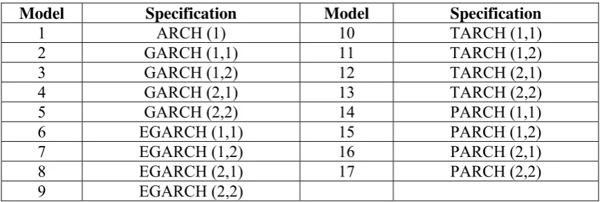
peso-dollar exchange rate from January 02, 1997 to December 05, 2003, a total of 1730 observations.

Table 1. Specification for ARCH-type Models *

Model Specification Model Specification

1 ARCH (1) 10 TARCH (1,1)

2 GARCH (1,1) 11 TARCH (1,2)

3 GARCH (1,2) 12 TARCH (2,1)

4 GARCH (2,1) 13 TARCH (2,2)

5 GARCH (2,2) 14 PARCH (1,1)

6 EGARCH (1,1) 15 PARCH (1,2)

7 EGARCH (1,2) 16 PARCH (2,1)

8 EGARCH (2,1) 17 PARCH (2,2)

9 EGARCH (2,2)

* The 17 models are estimated via the MLE using the Gaussian, Student’s t and the Generalized Error Distribution and using the QMLE resulting to 68 models.

Following the approach of Hansen and Lunde (2001), the time series was divided into two sets, an estimation period and an evaluation period.

t ₁₄₂₄₃K _{1 K4243}

period evaluation period

estimation

n T +1, ,0 1,2, ,

− =

The parameters of the volatility models are estimated using the first T inter-daily observations and the estimates of the parameters are used to make forecasts of the remaining n periods. The estimation period made use of daily returns from January 02, 1997 to December 27, 2002, a total of 1493 observations. In the evaluation period the daily volatility is estimated using the square of the Parkinson Range. The square of the PARK-R serves as the proxy for the unknown conditional variance. The evaluation period makes use of daily returns from January 02, 2003 to December 05, 2003, a total of 237 observations.

3.2. Measures to Evaluate the Forecasting Performance

The main objective of building volatility models is to forecast future volatility. Given a number of competing models, there is a need to evaluate the forecasting performance of the models to segregate “good” models from “bad” ones. This section discusses some of the commonly used measures to evaluate the forecasting performance of the volatility models. Let h denote the number of competing forecasting models. The jth model provides a sequence of forecasts for the conditional variance,

h j

n j j

j ,ˆ , , ˆ 1,2, ,

ˆ2_,1 σ2_,2 K σ2_, = K

σ

that will be compared to the square of the Parkinson range, the proxy of the intra-daily calculated volatility,

n P

P R

The forecast of jth model leads to the observed loss,

237 ,..., 2 , 1 68

,..., 2 , 1 )

, ˆ ( 2_, 2

, R j = and t=

L

t P t j t

j σ

In this study, five (5) different loss functions are used to evaluate the forecasting performance of the different models. The loss functions are based on the mean absolute deviations using the estimated conditional standard deviation (MAD1) and variance (MAD2), mean square error based on the conditional standard deviation (MSE1) and variance (MSE2) and a criterion equivalent to the R2 criterion using the regression equation,

237 , , 2 , 1 )

ˆ log( )

log(R2 =a+b _t2 + _t t= K

t

P σ ε

discussed in Engle and Patton (2001) and Taylor (1999).

3.3. Empirical Results

The best over-all ARCH model is the TARCH (2,2) model with the Student’s t as the underlying distribution. The second “best” model is the PARCH (2,2) model, also using the Student’s t distribution. It is interesting to note that models using the Generalized Error Distribution performed relatively well using the five forecasting criteria, with 8 out of 17 models landing in the top 10 models. In general, the models with relatively superior forecasting performance, using the peso-dollar exchange rate, are those that accommodate the leverage effects such as the TARCH, PARCH and EGARCH. However, while the correct specification of the volatility is important, one must also consider the distribution used in estimating the parameters of the model.

The results of the empirical analysis showed that volatility models that assumed the Gaussian distribution or those that used the QMLE performed worst compared to models that assumed the Student’s t or Generalized Error distributions. Therefore, it is important to correctly specify the entire distribution and not only to focus on the specification of the volatility, even if it is the object of interest. A similar observation was made in the study of Hansen and Lunde (2001).

IV. CONCLUSIONS

This study compared a large number of ARCH-class of volatility models using inter-daily returns of the peso-dollar exchange rate. The estimated models are compared in terms of their out-of-sample forecasting performance to characterize the variation in the volatility. The Parkinson Range is used as the estimate of the daily volatility where comparison of the different volatility models was made. The empirical analysis showed that it is important to correctly specify the entire distribution of the volatility model and not only focus on the specification of the volatility.

The Philippine Statistician, 2004 9

ACKNOWLEDGEMENT

The author wishes to thank Professors Adolfo M. De Guzman, Lisa Grace S. Bersales and Joselito C. Magadia for their comments and suggestions. All remaining errors are the author’s responsibility.

References

ANDERSEN T.G. and BOLLERSLEV, T. (1998), “Answering the Skeptics: Yes, Standard Volatility Models do Provide Accurate Forecasts”, International Economic Review, 39, 885-905.

ANDERSON, T., BOLLERSLEV, T., DIEBOLD, F. X., and LABYS, P. (2001), “Modeling

and Forecasting Realized Volatility”, working paper 8160, National Bureau of Economic Research, March 2001.

BARNDORFF-NIELSEN, O. E. and SHEPHARD, N. (2002), “Estimating Quadratic Variation using Realized Variance”, Journal of Applied Econometrics, 17, 457-477.

BLACK, F. (1976), “Studies of Stock Price Volatility Changes”, Proceedings from the American Statistical Association, Business and Economic Section, 177-181.

BOLLERSLEV, T. (1986), “Generalized Autoregressive Conditional Heteroskedasticity”, Journal of Econometrics, 31, 307-327.

BOLLERSLEV, T. and WOOLDRIDGE, J. M. (1992), “Quasi Maximum Likelihood Estimation and Inference in Dynamic Models with Time Varying Covariances”, Economic Reviews, 11, 143-172.

CAMPBELL, J. Y., LO, A. W., and MACKINLAY, A. C. (1997), The Econometrics of

Financial Markets. USA: Princeton University Press.

DING, Z., ENGLE, R.F., and GRANGER, C. W. J. (1993) “Long Memory Properties of Stock Market Returns and a New Model”, Journal of Empirical Finance, 1, 83-106.

ENGLE, R. F. (1982), “Autoregressive Conditional Heteroscedasticity with Estimates of the Variance of United Kingdom Inflation”, Econometrica, 50, 987-1007.

ENGLE, R. F. and PATTON, A. J. (2001), “What Good is a Volatility Model?” unpublished manuscript, Department of Finance, Stern School of Business, New York University.

GLOSTEN, L. R., JAGANNATHAN, R., and RUNKLE, D. (1993) “On the relation between the Expected Value and the Volatility of the Nominal Excess Return on Stocks”, Journal of Finance, 48, 1779-1801.

LEE, S. and HANSEN B. E. (1994), “Asymptotic Theory for the GARCH (1,1) Quasi-Maximum Likelihood Estimator”, Economic Theory, 10, 29-52.

LUMSDAINE, R. L. (1996), “Consistency and Asymptotic Normality of the Quasi-Maximum Likelihood Estimator in IGARCH (1,1) and Covariance Stationarity GARCH (1,1) Models”, Econometrica, 64, 575, 596.

NELSON, D. (1991), “Conditional Heteroskedasticity in Asset Returns: A New Approach”, Econometrica, 59, 347-370.

PARKINSON, M. (1980), “The Extreme Value Method for Estimating the Variance of the Rate of Return”, Journal of Business, 53, 61-65.

TAYLOR, J. W. (1999), “Evaluating Volatility and Interval Forecasts”, Journal of Forecasting, 18, 11-128.