Removal of Random Valued Impulse Noise by
Directional Mean Filter Using Statistical Noise based
Detection
1R. Seetharaman
2R. Vijayaragavan,
1
Department of ECE,College of Engineering Guindy,Anna University, Chennai, India.
2
Department of ECE,National Institute of Technology Tiruchirappalli, India.
ABSTRACT
Digital image processing and video processingare mainly used for the noise removal technique is a highly demanded research field.The main objective of this paper work is to detect and de-noise the image using a novel two stage algorithm for the removal of random valued impulse noise from the images is presented.In this paper, the first stage does the noise pixels are detected using the average deviations and threshold value. In the second stage,the directional differences between the four main directions are calculated. The median values of the pixels which lie in the direction of minimum difference are calculated and the noisy pixel values are replaced with the median value. This method identifies the noisy pixels in the corrupted images. So the two stage algorithm for image denoising random valued impulse noise is used. Experimental results show that proposed method is superior to the conventional methods in Peak Signal Noise Ratio (PSNR) values of the image performs, with and without noise compared. Comparison of PSNR values of the proposed method and the existing techniques show that the proposed method perform better than the existing one.
Index terms
Impulse noise,random valued impulse noise,noise detection, Image De-noising, Nonlinear Filters.
1. INTRODUCTION
Noise removal and suppression from images is one of the most important techniquesconcerns in digital image processing. The impulse noise is one of the most important noise, which comes from duringtransmission time errors in analog to digital conversion processing time. An important characteristic of this type of noise is that only a part of the pixels are corrupted and the remaining part noise-free.Fixed valued impulse noise takes the values 0 and 255 where as the random valued impulse noise takes the values in the dynamic range of [0,255]. Various methods have been proposed in the literature for the removal of random value impulse noise.
One of the important most efficient methods is the median filter method.This method is mainly used tosuppress noise with highcomputational efficiency. However, since using the technique, average of the every pixel in the image is replaced by the median value in itsconsider for the neighborhood value. The median filter often removes desirable details in the noise image and blurs image it too. The weighted median filter and the center-weighted median filter were proposed as to improve the median filter by giving more weight to some selected pixels in the filtering window. Although these two filters can preserve more details than the median filter, they are still implemented uniformly across the image without considering whether the current pixel is noise-free or
to a pixel value to its four most similar neighbors. Consider the noise level is high it introduces that time introduces blurring in the image.The methods which filters all the pixels irrespective of the corruption noise to blur the image, hence the techniques which follow the two stage process of detection of noise pixels and filtering of noise pixels are employed to achieve better performance in terms of peak signal to noise ratio.In order to overcome the difficulties in this paper, a two stage algorithm removal of impulse noise is proposed. The proposed method is simple and outperforms the existingmethods in terms of the peak signal to noise ratio.
2. TWO STAGE ALGORITHM FOR
REMOVAL OF IMPULSE NOISE
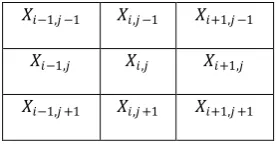
Consider X to be a random valued noise corrupted image of sizeMxN and X(i,j) denote the grey level at the pixel location (i,j). The pixels in the detection window „P‟of size 3x3 is denoted asP= [𝑋𝑖−1,𝑗 +1, 𝑋𝑖,𝑗 +1, 𝑋𝑖+1,𝑗 +1, 𝑋𝑖−1,𝑗
𝑋𝑖,𝑗, 𝑋𝑖+1,𝑗, 𝑋𝑖−1,𝑗 −1,𝑋𝑖,𝑗 −1,𝑋𝑖+1,𝑗 −1] (I)
In the first stage the noise corrupted pixels are detected using the absolute deviation between the mean value and the centre pixel value and by comparing with threshold value. In the second stage, the detected noise pixels are replaced with the median value of the pixels lying in the direction of the minimum difference.
2.1 Noise detection
Step 1: A 5x5 sliding window (p) was chosen from the noise corrupted image, and it runs from the top most left corner tothe bottom most right corner, covering the entire size of the image. The centrepixel of the 5x5window was treated as the test pixel.
Step 2:Usually the pixels located in the neighbourhood of a test pixel are correlated to each other and they process almost similar characteristics if the test pixelunder consideration is noise free. The absolute difference between the mean value and the centre pixel value in the chosen 5X5 window is calculated.
Step 3:Calculation of mean value.
µ =mxn1 mi=1 nj=1Xi,j (1)
wheremxn is the size of the chosen window.
Step 4: Calculation of the absolute deviation between the mean value and the centre pixel value.
Where 𝑋𝑖,𝑗 is the the centre pixel value in the 5x5windowunder consideration.
Step 5: The threshold value „T‟ is determined from each 5x5 window, to identify the pixelscorrupted by the noise. An adaptive thresholdvalue was calculated from each 3x3 window using the following equation to obtain the precise result.
T = 0.78 *σ (3)
Where „σ‟ is the standarddeviation for the 5x5 window under consideration
Step 6: Calculation of standard deviation.
σ = sqrt 𝑚𝑥𝑛1 𝑚𝑖=1 𝑛𝑗 =1(𝑋𝑖,𝑗−µ)2 (4)
Step 7: The pixel under consideration is treated as noisy pixel if the absolute deviation is greater than the threshold value otherwise the pixel istreated as noise free.
Step 8: Steps 3 to 7 are repeated until entire pixels in the noisy image „X‟ are covered.
Step 9: Binary noise mask „N‟ is created on the basis of step 8.
N i, j = 1, if d < 𝑇0, otherwise (5)
Step 10: Noise free pixels are sited directly to output image and Noisy pixels are subjected to filtering process.
2.2 Filtering stage
In this stage the “noise pixels” marked with N(i,j) = 0 is replaced by an estimated correction term.
[image:2.595.362.501.71.147.2]Step 1: Consider a 3x3 window, starting from the top-most left corner of the impulse noise corrupted image X.
Fig 1: A 3x3 window of noisy image
Step 2: The absolute differences between the current pixel and its neighbors in the four main directions (i.e.) horizontal, vertical and direction along two diagonals are calculated.
Dk(i, j) = |X(i+u, j+v) − X(i−u, j-v)| (6)
where, (k, u, v) = {(1, 1, 1), (2, 0, 1), (3,−1, 1), (4,−1, 0)}
Step 3:The direction along which the pixels giving the minimum difference valueis calculated (i.e.) Min {D1, D2, D3,
D4}.
Step 4: The median value of the pixels in the step 3 was calculated.
Step 5: Finally, the correction term to restore a detected “noise pixel” was obtained from the step 4 is replaced with the noise pixel value. The above steps 1 to5are repeated for all the pixels in the image.
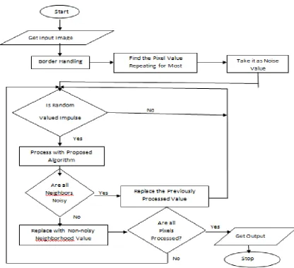
The flow chart shows the flow in which the image is processed. Get the image as input. Using border handling technique, find the pixel value. Repeating it for most, take it as a noise value. This value is checked against random valued impulse. If it is yes, then the value is processed with proposed algorithm. If it is no, then it is replaced with the previous value. Then the neighbours are checked for noise. If the neighbours are noisy then it replaced with the previously processed value. If the neighbours are non- noisy values, then it replaced with the same. This is repeated for all pixels and finally the output is arrived.
𝑋𝑖−1,𝑗 −1 𝑋𝑖,𝑗 −1 𝑋𝑖+1,𝑗 −1
𝑋𝑖−1,𝑗 𝑋𝑖,𝑗 𝑋𝑖+1,𝑗
Fig 2: Flowchart of Noise removal method
3. RESULTS AND DISCUSSSION
In this section, the feasibility of theproposed algorithm is compared to the other filters based on the quantitative measures. The PSNR (dB) evaluation scheme is used to access the strength of the filtered image, taken into consideration as to measure the computational efficiency of the filter implemented.In order to validate the proposed algorithm, Lena 512 ×512 png, 8- bit image is used in the analysis of the proposed algorithm which has been implemented on the MATLAB platform. This standard test image contains various characteristics suitable to test the performance of the filter being implemented.
Table 1 : Comparative PSNR Values of Various Filters on Noisy Lena Image.
Image /ND 10% 20% 30% 40% 50% 60%
Lena 36.07 35.17 32.71 31.2
6 28.6
8
24.77
peppers 37.13 36.91 35.44 34.1
5 31.7
1
27.92
barbara 24.06 23.75 23.05 22.8
0 22.3
8
21.68
boat 27.02 26.47 25.83 25.0
8 24.3
6
[image:3.595.298.550.550.661.2](a)
(b)
(c) (d)
(e) (f)
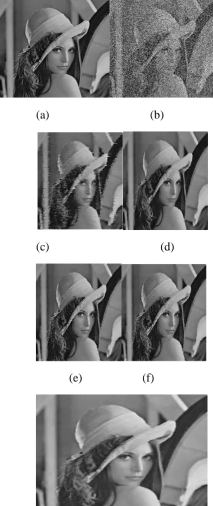
Fig 3: (a) original image (b) corrupted image (RVIN 40%) Restored image using (c) median filter (d) ROAD (e)
CWMF (f) PWMAD (g) proposed algorithm.
[image:4.595.54.267.73.578.2]Restoration results are quantitatively measured by peak signal-to noise ratio (PSNR), Table1 shows the PSNR values of the best results obtained by the proposed algorithm for the
Table 2:Comparative PSNR Values of Various Noise Filters on Noisy Lena Image.
filters. By experimental results, the performance of the proposed algorithm is better than the competing filters in terms of the peak signal to noise ratio. It also removes most of the noise while preserving the edge details very well, and even thin lines.
4. CONCLUSION
The proposed algorithm deals with the removal ofrandom valuedimpulsive Noise. Impulsive noise being contaminated in some pixels based on probability densities. The detector utilises a threshold value to compare with a predefined parameter. Fixed threshold is not suitable and do not work well under different noise conditions as well as for different images. In this algorithm, adaptive threshold determination strategy based on given noisy image statistics is proposed. Various statistical parameters i.e. (μ,𝜎2) are also used to predict the threshold value. The proposed filter is an impulsive noise removal scheme using the directional pixel wise difference method, replacing the corrupted pixel with the median value of pixels lying in the direction of minimum directional difference. The restored image, by this scheme exhibits the desirable properties of edge and detail preservation.Extensive simulations and comparisons are done with competent schemes. It is observed, in general, that the proposed schemes are better in terms of peak signal to noise ratio suppressing impulsive noise at different noise densities than their counterparts.
5. REFERENCES
[1] X. Zhang and Y. Xiong. 2009. Impulse noise removal using directional difference based noise detector and adaptive weighted mean filter. IEEE Signal Process.Lett., Vol. 16, no. 4, (Apr. 2009) pp. 295–298.
[2] Y. Dong and S. Xu. 2007. A new directional weighted median filter for removal of random-value impulse noise. IEEE Signal Process.Lett., vol. 14, pp. 193–196. Noise
density
Median ROAD CWMF PWMAD PA
10 31.56 34.45 34.73 31.23 36.07
20 30.23 32.09 33.07 30.09 35.17
30 28.05 31.01 32.56 26.45 32.71
40 24.61 28.94 28.79 22.65 31.26
[image:4.595.322.549.110.258.2]information. IEEE Trans. Image Processing, Vol. 12, pp. 85 -92.
[6] S. J. Ko and Y. H. Lee. 1991. Center weighted median filters and their applications to image enhancement. IEEE Trans. Circuits Syst., vol. 38,pp. 984–993.
[7] D. Brownrigg. 1984. The weighted median filter.Commun. Assoc. Comput.Mach., vol. 27, pp. 807– 818.
[8] Crnojevi.C.V, Senk.Vand Trpovski.Z 2004. Advanced impulse detection based on pixel-wise MAD. IEEE Signal Processing Letters, Vol. 11,No. 6, pp. 589–592..
[9] Chui.C, Garnett.R, Huegerich.T, and He.W.2005. A universal noise removal algorithm with an impulse detector. IEEE Trans on Image Processing, Vol. 14,No. 5, pp. 1747–1754.
[10] Ko .S.J. and Lee S.J., 1991.Adaptive centre weighted median filters and their applications to image enhancement. IEEE Transactions on Circuits and Systems, Vol. 15, No. 6, pp. 984–993.
[11] Bovik A. C. 2000. Nonli near filtering for image analysis and enhancement.Handbook of Image & Video Processing. San Diego,CA: Academic, ch. 3.2 (G. R. Arce), pp. 95–95.
[12] Alliney S and Morandi C. 1986. Digital image registration using projections.IEEE Trans. Pattern Anal. Mach. Intell., Vol. 8, No. 2, pp. 222– 233.