Probability Modeling of Multi Node Wireless Networks

(1)

Probability Modeling of Multi Node Wireless Networks

Suresh R. Halhalli

Associate Professor M.S Bidve Engineering College, Latur (MS)-India

Subhash Kulkarni

Principal, J.P.N College of Engineering Mahabubnagar (AP)-India

K.S.R Anjaneyulu

Director i/c, R & D Cell JNTUA Anantapur (AP)-India

S. Akhila

Associate Professor, BMS College of Engineering,

Bangalore (KS)-India

ABSTRACT

In this work, probability equations are derived for the five node networks and the probabilities are computed for unnecessary handover, missing handover and wrong decisions. Wrong decision probability is the summation of unnecessary and missing handover probabilities. Also, the handover probability is computed for the bandwidths up to 20. The modeling is based on the five state Morkov chain model. Simulations are carried out for the different decision times from D=1 to D=5 ms. The simulation results for the five node network model is compared with the two node and three node network models.

Keywords

Wrong Decision Probability, Missing Handovers, Unnecessary handovers.

1. INTRODUCTION

Vertical handover is very popular in the field of wireless communication due to the versatility it provides. Connectivity switching from a serving network to a candidate network [1] may be called as a vertical handover. Usually the parameters like received Signal Strength (RSS) [1], link-layer parameters such as bandwidth, delay, signal-to-noise ratio [2], as well as quality of service (QoS) [3] are used in the decision making of vertical handover. An overview of main decision metrics is described in [4]. The number of vertical handovers is another performance issue [5] and is a big limitation in this case. Mobile terminal’s battery life and the quality of service level is affected due to “ping pong effect” which may described as the switch over of mobile terminal repeatedly between two access network. There are several techniques available to limit vertical handovers, and hence the ping-pong effect [6, 7]. Handover probability modeling is gaining popularity and vertical handover analytical methods based on handover probability are explained in [8-9]. Wrong decision probability modeling for vertical handover decision is presented in [10]. In ref [10] authors adopted the wrong decision probability as a metric for vertical handover decision based on network parameters and one such metric used in this case was bandwidth. Wrong decision probability is also assumed as a performance metric for the proposed algorithms. The wrong decision probability is based on maximum capacity and available bandwidth from a candidate network. Wrong decision probabilities are evaluated for a sample capacity and available bandwidth and it is not the scope of the present work how wrong decision probability affects mobile terminal’s performances in terms of Quality of Service.

In [11], wrong decision probability, unnecessary handover probability and missing handover probability models are used

to predict the probabilities for different decision times and large bandwidth channels. The probability equations are derived in [11] was based on a two node network model. The traffic load of each network was varied based on the maximum band width available in the network node located in busy areas of cities and the probabilities of the handover, missing handover and unnecessary handovers are computed. Simulated results are presented for large bandwidth cases as well as for different decision times and important conclusions are drawn.

In [12] wrong decision probability modeling has been used to predict the probabilities of missing handovers and unnecessary handovers for different decision times, different bandwidths and larger number of available networks for performing handover leading to an increase in the throughput. The focus is laid on minimization of wrong decision probability. There is significant improvement in the reduction of wrong decision making when two network models is replaced by a three network model and also the ping-pong effect caused due to unnecessary handoff has been reduced which indicates that with increase in choice of neighboring networks effect of wrong decision probability can be minimized but with an obvious tradeoff between cost and number of networks. Further, parameters like Signal Strength and Mobility is considered for analyzing the effect of wrong decision probability on handover decision algorithms. In [13] the performance of a bandwidth, signal strength and bandwidth plus signal strength based handover algorithms for wrong decisions were studied. The simulated results show that considering both signal strength and network bandwidth is more advantageous to the network operator due to the reduction in the number of wrong decisions. Making handover decisions based on the predication method called wrong decision probability can provide better performance of the algorithm.

(2)

2. ANALYTICAL MODEL

Fig. 1 shows the layout of a network having five nodes

n

₁, 2

n

,

n

₃,

n

₄ and

n

₅; and the maximum available bandwidth for the two networks are

B

₁,

B

₂,

B

₃,

B

₄ and

B

₅

respectively. Let

ni nj

P

: The probability of mobile node moving from node

n

_i

to

n

_j.

ni ni

P

: The probability of mobile node continues to stay in

i

n

after a time interval D.

         



  5 1 / 1 i j j nj ni ni

ni P

P

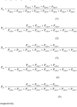
The five node network model can be treated as a five state Morkov model and the probabilities that a mobile node stays at

n

₁,

n

₂,

n

₃,

n

₄ and

n

₅can be expressed as

1 5 5 1 1 4 4 1 1 3 3 1 1 2 2 1 5 1 4 1 3 1 2 1 1 n n n n n n n n n n n n n n n n n n n n n n n n n P P P P P P P P P P P P P            (1) 2 5 5 2 2 4 4 2 2 3 3 2 2 1 1 2 5 2 4 2 3 2 1 2 2 n n n n n n n n n n n n n n n n n n n n n n n n n P P P P P P P P P P P P P            (2) 3 5 5 3 3 4 4 3 3 2 2 3 3 1 1 3 5 3 4 3 2 3 1 3 3 n n n n n n n n n n n n n n n n n n n n n n n n n P P P P P P P P P P P P P            (3) 4 5 5 4 4 3 3 4 4 2 2 4 4 1 1 4 5 4 3 4 2 4 1 4 4 n n n n n n n n n n n n n n n n n n n n n n n n n P P P P P P P P P P P P P            (4) 5 4 4 5 5 3 3 5 5 2 2 5 5 1 1 5 4 5 3 5 2 5 1 5 5 n n n n n n n n n n n n n n n n n n n n n n n n n P P P P P P P P P P P P P            (5) respectively.

3. GENERAL ALGORITHM

[image:2.595.313.547.72.257.2]

When mobile node decides to move from one network node to another node it is necessary that available band width in the new node is greater than a than by a threshold over the available bandwidth of current node. The value of the threshold value can be set to either zero or a positive integer.

Figure 1: Five state Markov Model

Following list of steps describe the algorithm designed in this work:

1. Assume that mobile node in the network node 1

n

and wants to move to another node. Assuming the network nodes

n

₂,

n

₃,

n

₄ and

5

n

can serve the area where the user wants to move to.

2. Define the threshold value as L.

3. If the mobile node is at

n

₁, then decision is made to switch over when

b

2 

b

1 

L

, 4. Else verify b3b1L and switchover to

n

₃ if

L b

b3 1 is true.

5. Else verify

b

4 

b

1 

L

and switchover to

n

₄ if L

b

b4 1 is true.

6. Else verify b5b1L and switchover to

n

₅ if L

b

b5 1 is true. 7. Else maintain the status quo. Or, the following algorithm may be followed.

1.Assume that mobile node in the network node

n

₁

and wants to move to another node. Assuming the network nodes

n

₂,

n

₃,

n

₄ and

n

₅ can serve the area where the user wants to move to. 2.Define the threshold value as L.

3.If the mobile node is at

n

₁, then decision is made to switch over when



b

2 |

b

3 |

b

4 |

b

5 



b

1 

L

, 4.Switch over to

n

_i based on

max

 

b

_i

5.Else maintain the status quo.

Practically the available bandwidth of any network keeps changing dynamically, and sometimes rapidly. However, in this case for ease of simulations, the bandwidths of the networks are assumed to be static. All the analytical expressions listed in the previous section are based on the general algorithm defined above.

[image:2.595.53.305.339.688.2]

(3)

Hence,



bi

bj

L



P

ninj



Pr





(6)

Handover probabilities for such an arrangement are given by













































5 4 5 3 5 2 5 1 5 4 5 4 3 4 2 4 1 4 3 5 3 4 3 2 3 1 3 2 5 2 4 2 3 2 1 2 1 5 1 4 1 3 1 2 1

5

1

n n n n n n n n n n n n n n n n n n n n n n n n n n n n n n n n n n n n n n n n n n n n n

P

HP

(7)

Let, the probability of occupied bandwidth is given by







i B 0 j j i k i k , i

!

j

!

k



(8)

Sterling’s approximation can be used to compute the factorials of large numbers, which is given by

n

e

n

2 !

n

















(9)

If the arrival rate of requests channels follows a Poisson’s distribution with parameter



_i and service rate is given by



i



i





B



k

/

B



(10)

4. UNNECESSARY HANDOVER

For a five node network, probability of unnecessary handover can be expressed as

























k

r

D

 

D

r

k

P

D

r

k

D

r

k

P

D

r

k

D

r

k

P

UHP

B m B L m k k B m B B L j L j k k B j B n n n B i B L i k k B i B B L m L m k k B m B n n n B i B L i k k B i B B L j L j k k B j B n n n

,

...

,

...

,

5

1

4 0 , 4 , 5 5 0 , 5 , 4 5 4 5 5 0 , 5 , 1 1 0 , 1 , 5 1 5 1 2 0 , 2 , 1 1 0 , 1 , 2 1 2 1 5 2 4 5 5 5 4 1 3 5 1 5 1 5 1 2 2 1 2 1 2















                           

























(11) where









m k r





D

0 s s i D k B 0 m m i

i i i

i e ! s D e ! m D D , k ,

r







      



  (12) and













                 



m k r D

0 s s i D k B 0 m m i

i i i

i e ! s D 1 e ! m D D , k ,

r







.

(13) MATLAB code is used to compute the probability for the unnecessary handover is computed and the results are depicted in this section. Simulation results presented for the cases where the maximum channel bandwidths are 21 and decision time are 1 to 5 ms. The values for the bandwidth and decision time are indicative only and these values need to be taken from a real network when computing the probabilities of physical networks.

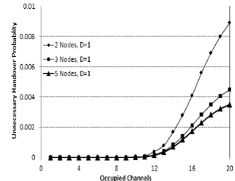
[image:3.595.315.551.440.621.2]

Probabilities are computed for similar conditions like the maximum bandwidth available, decision time and threshold value for a five node network. Fig 2 shows the comparison of the probabilities for the network models with 2 nodes, 3 nodes and 5 nodes for a case with decision time of 1 ms. It is clear from the plots that there is a good amount of reduction in the unnecessary handover based on the probabilities computed when the number of network nodes increase from 2 to 5.

Figure 2: Unnecessary Handover Probability Vs Occupied number of channels for 2 node, 3 node and 5 node network

(4)

[image:4.595.64.269.67.234.2]

Figure 3: Unnecessary Handover Probability Vs Occupied number of channels for 2 node, 3 node and 5 node network

models for D = 3 ms.

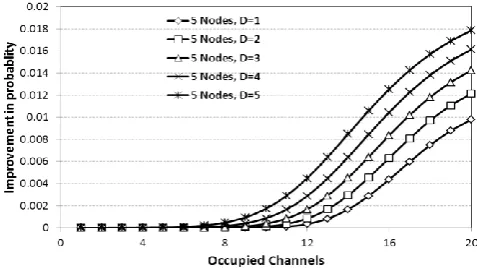
[image:4.595.66.270.500.643.2]

Similarly, Fig. 3 shows the unnecessary probabilities for the 2 node, 3 node and 5 node networks for the case with a decision time of 3 ms. Fig. 4 shows the improvement (reduction) in the unnecessary probability by changing the network model from 2 node networks to 3 node networks and from 3 node to 5 node networks. Though higher decision times result in higher probabilities of unnecessary handover probabilities, it also results in higher reduction in the unnecessary handovers. Similarly for the same decision time, there is a significant reduction of unnecessary handover as the occupied number of channels increase. It can also be concluded from Figs. 2, 3 and 4 that, with increase in decision time, the probability of unnecessary handover increase for all the three networks. It is obvious that with more delay in the decision making, more the probability that the available bandwidth in the present network changes. However, the plot above quantifies the probabilities.

Figure 4: Unnecessary Handover Probability Vs Occupied number of channels for 2 node and 3 node network models

for D = 1 to 5 ms.

5. MISSING HANDOVER

For a three network model, probability of missing handover can be expressed as





































 

.

,

1 ...

,

1 ...

,

1

3

1

5

1 1

, 5 ,

4

4 0

1 0

, 4 ,

5 5 4 5

1

1 1

, 1 ,

5

5 0

1 0

, 5 ,

1 1 5 1

1

1 1

, 1 ,

2

2 0

1 0

, 2 ,

1 1 2 1

4 5

5 4

5

4 5

5 1

1 5

1

5 1

2 1

1 2

1

2 1

D

r

k

D

r

k

P

D

r

k

D

r

k

P

D

r

k

D

r

k

P

MHP

B

L j

B

L j k

k B j

B B

m

L m

k

k B i

B n

n n

B

L m

B

L m k

k B m

B B

i

L i

k

k B i

B n

n n B

L j

B

L j k

k B j

B

i

L i

k

k B i

B n

n n

















     



 

 

 

     



 

 

 

     



 

 

































(11) where









m k r





D

0 s

s i D

k B

0 m

m i

i i i

i

e ! s

D e

! m

D D

, k ,

r







  

 











(12) and













    

  

 

   

 







m k r D

0 s

s i D

k B

0 m

m i

i i i

i

e ! s

D 1

e ! m

D D

, k ,

r







. (13)

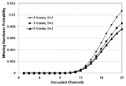
The probability for the missing handover is computed using MATLAB code and the results are presented in the following plots. Simulation results presented for the cases where the channel bandwidths are 21 and decision time are 2 and 4 ms. Again, two networks are modeled in this work, namely, 2 node network and 3 node network for computing the missing handover probabilities based on the work presented by ref [11-13]. For both of these network models, probabilities are computed for similar conditions like the maximum bandwidth available, decision time and threshold value. Fig. 5 shows the comparison of the probabilities for the 2 node, 3 node and 5 node network models for a case with decision time of 2 ms. It is clear from the plots that there is a good amount of reduction in the missing handover based on the probabilities computed.

(5)

[image:5.595.70.287.74.222.2]

Figure 5: Missing Handover Probability Vs Occupied number of channels for 2 node and 3 node network models

for D = 2 ms.

[image:5.595.64.279.367.506.2]

Similarly, Fig. 6 shows the missing probabilities for the 2 node, 3 node and 5 node networks for the case with a decision time of 4 ms. Yet again, it can be concluded from Figs. 5 and 6 that, with increase in decision time, the probability of missing handover increase for both the networks. It is obvious that with more delay in the decision making, more the probability that the available bandwidth in the present network changes. However, the plot above quantifies the probabilities.

[image:5.595.59.277.370.669.2]

for D = 4 ms.

for D = 1 to 5 ms.

Fig. 7 shows the improvement (reduction) in the missing probability by changing the network model from 2 node network to 3 node network. Though higher decision times

result in higher probabilities of missing handover probabilities, it also results in higher reduction in the missing handovers. Similarly for the same decision time, there is a significant reduction of missing handover as the occupied number of channels increase.

6. WRONG DECISION PROBABILITY

Wrong decision probability is the summation of the unnecessary handover probability and missing handover probability, which is given by

MHP

UHP

WDP





(14)

[image:5.595.314.551.466.654.2]

Figs. 8, 9 and 10 shows the probabilities for the Wrong decision probability vs. the occupied number of channels when, the maximum channel band widths available in both the networks are 21. Wrong decision probability is the summation of unnecessary handover probability and missing handover probability as explained earlier. Higher the decision time, more the probability of wrong decision making.

Figure 8: Wrong Decision Probability Vs Occupied number of channels for 2 node and 3 node network models

[image:5.595.56.268.556.681.2]

for D = 1 ms.

(6)

[image:6.595.55.294.76.210.2]

[image:6.595.61.292.268.413.2]

for D = 1 to 5 ms.

Figure 11: Handover Probability

Fig. 10 shows the improvement (reduction) in the wrong decision probability by changing the network model from 2 node network to 3 node network. Though higher decision times result in higher probabilities of wrong decision probabilities, it also results in higher reduction in the missing handovers and unnecessary handovers. Similarly for the same decision time, there is a significant reduction of wrong decisions as the occupied number of channels increase. Computation of probabilities becomes difficult as the traffic density increases as it involves evaluation of the factorials. The factorials of large numbers are numerically very high values and its accurate computation is very difficult. The factorials of numbers which are beyond 150 cannot be computed using normal computers with 2GB RAM and 28 GHz processor. Hence, it poses a challenge to evaluate the expressions of the probabilities by different mathematical techniques, which is beyond the scope of present work.

7. CONCLUSIONS

In this work, probability models are used to predict the probabilities of missing handovers, unnecessary handovers and wrong decision for different decision times and large bandwidth channels for two network models, namely, 2 node, 3 node and 5 node networks. The probability equations are derived for all these network models. The occupied number of channels for each network is varied based on the maximum band width available in the network node located in busy areas of cities and the probabilities of the wrong decision, missing handover and unnecessary handovers are computed. It has been concluded that higher the decision time, more the probability of wrong decision making due to the obvious reason that with more delay in the decision making, more the probability that the available bandwidth in both the present

and other network changes which leads the wrong decision making. Similarly, there is significant improvement in the reduction of wrong decision making when two node network models is replaced by a three node network models and from three node network model to five node network model. Computational difficulties in evaluating the probabilities for the large bandwidth networks are explained along with limitations.

8. REFERENCES

[1] M. Ylianttila, M. Pande, J. Makela, and P. Mahonen 2001, Optimization scheme for mobile users performing vertical handoffs between IEEE 802.11 and GPRS/EDGE networks, in Proc. IEEE Globecom. [2] EURESCOM Project P1013-FIT-MIP, First steps towards

UMTS: Mobile IP services, a European testbed,

http://www.eurescom.de/public/projects/P1000-series/p1013/default.asp.

[3] J. McNair, I. Akyildiz, and M. Bender 2000, An inter-system handoff technique for the IMT-2000 inter-system, in Proc. IEEE infocom.

[4] C. Perkins, Editor, IP mobility support for IPv4,” RFC 3344, http://www.ietf.org/rfc/rfc3344.txt

[5] C. Perkins, et al. 2003, Mobility support in IPv6, IETF draft, http://www.ietf.org/internet-drafts/draft-ietfmobileip- ipv6-24.txt, work in progress.

[6] A. Valko 1999, Cellular IP: A New Approach to Internet Host Mobility,” Computer and Communication Review, vol. 29, no.1, pp. 50-65.

[7] R. Ramjee, et al 1999. HAWAII: A domain-based approach for supporting mobility in wide-area wireless networks, in Proc. IEEE ICNP.

[8] S. Aghalya, P. Seethalakshmi 2010, An Efficient Decision Algorithm for Vertical Handoff Across 4G Heterogeneous Wireless Networks, International journal of computer science and information security, vol8, no 7. [9]. Gabriele Tamea, Anna Maria Vegni, Tiziano Inzerilli, Roberto Cusani 2009, A Probability based Vertical Handover Approach to Prevent Ping-Pong Effect, The Sixth International Symposium on Wireles Communication Systems (ISWCS09)

[10] C. Chi, X. Cai, R. Hao and F. Liu 2007, Modeling and Analysis of Handover Algorithms, IEEE GLOBECOM proceedings.

[11] S. Akhila and Suthikshn Kumar 2010, Analysis of Handover Algorithms based on Wrong Decision Probability Model, International Journal of Wireless Networks and Communications, Volume 2, Number 3, pp. 165—173.

[12] S. Akhila and Suthikshn Kumar 2011, Reduction of Wrong Decisions for Vertical Handoff in Heterogeneous Wireless Networks, International Journal of Computer Applications (0975 – 8887) Volume 34– No.2.