Optimal hedging strategies for multi period guarantees in the presence of transaction costs: A stochastic programming approach

Optimal hedging strategies for

multi-period guarantees in the presence

of transaction costs: A stochastic

programming approach

Fleten, Stein-Erik and Lindset, Snorre

October 2004

Online at

https://mpra.ub.uni-muenchen.de/7645/

Optimal hedging strategies for multi-period guarantees

in the presence of transaction costs: A stochastic

programming approach

q

Stein-Erik Fleten

, Snorre Lindset

a_{Norwegian University of Science and Technology, Department of Industrial Economics and Technology Management,}

Alfred Getzvei 3, 7491 Trondheim, Norway

b_{Trondheim Business School, HIST avdeling TØH, 7004 Trondheim, Norway}

Abstract

Multi-period guarantees are often embedded in life insurance contracts. In this paper we consider the problem of hedg-ing these multi-period guarantees in the presence of transaction costs. We derive the hedghedg-ing strategies for thecheapest hedge portfolio for a multi-period guarantee that with certainty makes the insurance company able to meet the obligations from the insurance policies it has issued. We find that by imposing transaction costs, the insurance company reduces the rebalancing of the hedge portfolio. The cost of establishing the hedge portfolio also increases as the transaction cost increases. For the multi-period guarantee there is a rather large rebalancing of the hedge portfolio as we go from one per-iod to the next. By introducing transaction costs we find the size of this rebalancing to be reduced. Transaction costs may therefore be one possible explanation for why we do not see the insurance companies performing a large rebalancing of their investment portfolio at the end of each year.

Ó2006 Elsevier B.V. All rights reserved.

Keywords: Multi-period guarantee; Optimal hedging strategies; Transaction costs; Stochastic programming

1. Introduction

A life insurance company is mainly exposed to two types of risks; mortality risk and financial risk.

Mortality risk is the risk that a policyholder lives longer or dies earlier than what is expected. This is a risk that can, by the law of large numbers, be diversified away by issuing many similar policies. The premiums collected by a life insurance company are typically invested in the financial market. A typ-ical investment portfolio for an insurance company consists of bonds, stocks, and in some cases also real estate. The return on a life insurance policy is often a function of the return on the insurer’s investment portfolio. Since many policies have a minimum guaranteed rate of return included, the uncertain

0377-2217/$ - see front matter Ó_{2006 Elsevier B.V. All rights reserved.}

doi:10.1016/j.ejor.2006.08.013

q

First version:June 11, 2004.This version:April 7, 2006. The paper was presented at the World Risk and Insurance Economics Congress in Salt Lake City, Utah, USA.

*

Corresponding author. Tel.: +47 73 55 99 78.

E-mail addresses:stein-erik.fl[email protected](S.-E. Fleten),

[email protected](S. Lindset). 1 _{Tel.: +47 73 59 12 96.}

European Journal of Operational Research xxx (2006) xxx–xxx

www.elsevier.com/locate/ejor

return on the investment portfolio exposes the insurers to financial risk. In contrast to mortality risk, financial risk increases in the number of poli-cies issued. Thus, the financial risk is undiversifiable. To reduce the probability of bankruptcy, the financial risk should be integrated in the company’s overall risk management systems. In particular, the company should have a solid knowledge about how to hedge the financial risk inherent in the minimum rate of return guarantees.

Abstracting from mortality risk, a life insurance policy is basically a financial derivative that is writ-ten (on the return) on the life insurance company’s investment portfolio. In a complete market, all financial derivatives can be replicated by self-financ-ing tradself-financ-ing strategies, the market value of the life insurance contract included. In the absence of arbi-trage, it is clear that the market value of the insur-ance policy has to equal the initial cost of the replicating portfolio.

In this paper we focus on the hedging or replica-tion of a policy with a so-calledmulti-period guaran-tee embedded.2 In some countries the return on a life insurance contract is subject to an annual mini-mum guaranteed rate of return. For instance, if the annual minimum guaranteed rate of return is 4%, and the return on the insurance company’s invest-ment portfolio in year one and two are10% and 15%, respectively, the return on and the cash flow from the insurance policy develop as in Fig. 1 (assuming one unit of account is invested with the guarantee embedded).

The multi-period guarantee has a sort of ‘‘rat-cheting-effect’’, i.e., any good return in earlier peri-ods will not be lost in a period with a ‘‘low’’ return on the investment portfolio. It turns out that this type of guarantee is rather expensive and exposes the life insurance companies to a

consider-able amount of financial risk. The ‘‘delta’’ of the guarantee can be rather large and can be much lar-ger than one. It is therefore important that the issu-ers of such guarantees are aware of how to hedge them.

The hedging strategy for the multi-period guar-antee distinguishes it self quite a bit from the hedg-ing strategy for, say, a standard call option. From theBlack and Scholes (1973)analysis we know that the hedging strategy for a call option is a portfolio of the underlying stock and the risk free asset. The exact holdings of the two assets are given by Ito pro-cesses withcontinuous trajectories over the life time of the option. This is not the case for the strategy for the multi-period guarantee. This strategy experi-ences a discontinuity, or jump, as one goes from one period to the next. That is, there is either a signifi-cant sell-off of the investment portfolio or the risk free asset, this depending on whether the guarantee is binding or not. Of course, since the replicating portfolio is self-financing, a sell-off of the risk free asset leads to an increased holding of the investment portfolio, and vice versa.

In practice, one does not observe the insurance companies performing such a major rebalancing of their balance sheet at the end of each year. There can be several reasons for this. One is that the pol-icies they have issued are more complex than the one described above; another is that they do not cre-ate a perfect hedge for the guarantees they have issued. A third explanation, which is the one we investigate in this paper, is the presence of transac-tion costs. It is reasonable to expect that the volume of trading will diminish as the cost of trading increases. In particular, the focus in this paper is on the impact transaction costs have on the large rebalancing that is undertaken as we go from one period to the next.

The paper is organized as follows: in Section2we present assumptions underlying our economic model and the insurance policy. In Section 3 we review results regarding the hedging of the multi-period guarantee in the absence of transaction costs. In Section4we analyze the hedging strategies in the presence of transaction costs. Section5 concludes.

2. The economic model and the insurance policy

As argued in Section 1, mortality risk can be diversified by issuing many similar policies. We therefore abstract from this type of risk and instead concentrate on financial risk.

Fig. 1. The figure shows the return on and the cash flow from the insurance policy when one unit of account is invested in the insurer’s investment portfolio and a two-period guarantee is embedded.

2 _{Sometimes we refer to the insurance policy with a guarantee}

embedded as simplythe guarantee.

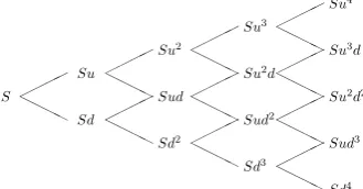
We assume a very simple model for the financial market. Only two ‘‘assets’’ are considered; the insur-ance company’s investment portfolio and a risk free asset. We assume that a binomial process gives the portfolio value. The market value of the investment portfolio isSiin nodei. In nodei+ 1, the portfolio

value has either increased to

Siþ1¼Siu ð1Þ

or decreased to

Siþ1¼Sid; ð2Þ

where

d ¼1

u; ð3Þ

see e.g.,Cox et al. (1979). This is also illustrated in Fig. 2 (here S0 is abbreviated to S). Let r be the

instantaneous standard deviation of the return on the investment portfolio in a continuous time model and let Dtbe the time interval between node iand

i+ 1. We then define the factoruas

u¼erpffiffiffiffi_Dt :

The risk free asset is a bank account accruing the constant short term interest rater= lnR, from one node to the next, thus

Biþ1¼BiR; ð4Þ

whereB0= 1.

For simplicity we assume the company only has issued one contract. The contract lasts for two peri-ods (each will typically be of one year). LetIbe an even number. We divide each period into I/2 time steps, i.e., nodeI/2 is the end of the first period (also the beginning of the second period), while nodeIis the last node in the second period. Letibe the num-ber of up-moves in the first period andjthe number of up-moves in the second period. The return on the investment portfolio in the first period is then defined as

d_1¼ui_dI=2i

1 ð5Þ

and for the second period

d_2¼uj_dI=2j

1: ð6Þ

In each period the policyholder is guaranteed a minimum rate of return equal tog. This is known as a multi-period guarantee, or in this case a two-period guarantee. There are several interpretations of this type of guarantee, but we choose the same interpretation as in e.g., Miltersen and Persson (1999), i.e., the contract with the two-period guaran-tee embedded has a terminal cash-flow at the end of the second period of (i.e., in nodeI)

p_2¼maxðD_{1;GÞ maxð}D_{2;GÞ; ð7Þ}

where D_{i= 1 +}d_{i, i2{1,2}, and G= 1 +g. To}

emphasize the fact that the policy has a guarantee embedded, we will throughout denote the policy

the guarantee.

As is evident from Eq.(7), the multi-period guar-antee is a path dependent derivative asset. The ter-minal payoff is dependent on the return on the investment portfolio in the different periods. This is illustrated inFig. 3 for the two-period guarantee when the investment portfolio evolves as in Fig. 2 and each period is of two time steps.

In a real world financial market, the trading of financial assets comes at a cost. Stockbrokers and other financial intermediaries charge their custom-ers a fee when selling and buying financial assets. For simplicity we assume that there is only a cost associated with trading the investment portfolio, not the risk free asset. As will become clear later, to hedge the guarantee, the company has to con-struct a hedge portfolio consisting of the investment portfolio and the risk free asset. The proceedings from a sale of part of the investment portfolio, net of transaction costs, will be invested in the risk free asset and cash needed to increase the holding in the investment portfolio will have to be raised by a reduction in the holding of the risk free asset. No infusion or withdrawal of cash from the hedge port-folio is allowed for.

Letai1be the number of units of the investment

portfolio in the hedge portfolio that we ‘‘arrive’’ in node i with, and ai the number we ‘‘leave’’ with.

The corresponding quantities for the risk free asset are given bybi1andbi, respectively. Total

transac-tion cost in nodeiis given by

Ci¼ jaiai1jSic; Fig. 2. Illustration of the development in the value of the

investment portfolio for four time steps.

S.-E. Fleten, S. Lindset / European Journal of Operational Research xxx (2006) xxx–xxx 3

for some parameter 06c< 1. Here c represents a proportional transaction cost. Thus, there are no fixed costs associated with rebalancing the hedge portfolio.

3. Hedging with zero transaction costs

The motivation for this paper is partially an observation inLindset (2003). It is there observed, although in a continuous time setting, that there is a large rebalancing of the hedge portfolio as we go from one period to the next. This discontinuity is illustrated inFig. 4.

In the case of zero transaction costs, it is straight-forward to create a perfect hedge of the guarantee. Let f(u) be the value of the guarantee in case the

investment portfolio has had an up-move from node

itoi+ 1 andf(d) for a down-move. We then need a hedging strategy satisfying Eqs. (8) and (9)

aiSiuþbiBiR¼fðuÞ ð8Þ

and

aiSidþbiBiR¼fðdÞ: ð9Þ

The solution to these two equations is

ai¼

fðuÞ fðdÞ

SiðudÞ ð

10Þ

and

bi¼

fðdÞ ðfðuÞ fðdÞÞd

ud BiR

: ð11Þ

0 0.2 0.4 0.6 0.8 1 1.2 1.4

Value investment portfolio Units of risk free asset period #2 Units of investment portfolio period #1 Units of investment portfolio period #2 Units of risk free asset period #1

Fig. 4. Illustration of the discontinuity in the replicating portfolio (for a continuous time model) as we go from the first to the second period.

Fig. 3. Illustration of the gross return on the two-period guarantee given the development in the value of the investment portfolio inFig. 2. (a_{_}b) = max(a,b).

Consider the situation where the investment portfolio has been performing badly in most of the first period, and any up-movements cannot pro-hibit the guarantee from becoming binding in the first period. This implies that3f(u)f(d) = 0, thus,

ai¼0 and bi¼

fðdÞ

BiR :

Similarly, if the investment portfolio has been per-forming well and any down-movements cannot make the guarantee become binding in the first per-iod, we have that f(u)f(d) =Si(ud)h, thus, ai¼h and bi¼0:

Here h _{is the time 1 market value of a guarantee}

with time 2 payoff pm

2 ¼maxðD2;GÞ. This basically

follows sinceD_1andD_{2are statistically independent.}

However, in the beginning of the second period, bothaiandbiwill be strictly positive if we exclude

contract specifications whereG>uI/2(the guarantee is always binding) orG<dI/2(the guarantee is never binding). We therefore conclude that there will also be a ‘‘large’’ change in the hedge portfolio as we go from the last node in the first period to the begin-ning of the second period.

4. Hedging with transaction costs

In this section we want to analyze the situation where we have a proportional transaction cost. It is reasonable to assume that it is more costly to rebalance the investment portfolio than it is to buy or sell the risk free asset. The costs may be both direct and indirect. The direct costs are such as com-mission fees to brokers and so on. For an insurance company with a large investment portfolio, the rebalancing of the investment portfolio may also have an influence on the liquidity in the market and represent an indirect cost. The total transaction cost may therefore be rather large.

That no transaction costs are imposed on selling or buying the risk free asset can also be justified by the fact that, for instance, any proceedings from selling parts of the investment portfolio, net of transaction costs, is used to buy the risk free asset. Therefore,ccan be interpreted as also incorporating the costs associated with buying or selling the risk free asset. Also, as pointed out byBoyle and Vorst (1992), including transaction costs on the trading of

the risk free asset, ‘‘_{. . .}the model becomes much more complicated without providing new insight.’’

By imposing this transaction cost on the rebalanc-ing of the hedge portfolio, we expect that less tradrebalanc-ing will take place than with zero transaction costs. In particular, what we would like to investigate in this paper is if the heavy rebalancing of the hedge portfo-lio at the end of the first period is still present when such a rebalancing is costly. And if so, does an increase in the cost of trading affect the hedge portfo-lio, and in particular, the size of the rebalancing at the end of the first period. When the management of the insurance company is trying to maximize the profit of the company, the cost of this rebalancing should be taken into account in their risk management routines. From standard corporate finance literature we know that the only goal that should be pursued by the management is to maximize the value of the share-holders’ stocks. Insurance companies are also subject to rather strict regulations. Here we assume that the insurer has to be able to meet the obligations imposed by the guarantee in every state of the world. The insurer does therefore have to create a hedge portfolio that will prevent it from defaulting on its obligations with certainty.4To maximize the market value of the share holders stocks, the management has to mini-mize the costs of establishing the hedge portfolio.5

LetH_{be the set of all possible trading strategies.} We take a andb to be the trading strategy for the investment portfolio and the risk free asset, respectively.

The insurer’s hedging strategy is the solution to the following optimization problem (for an introduc-tion to stochastic programming, see e.g., Kall and Wallace, 1994).

min

a;b2Hða0Sþb0Þ

subject to

aI1SIþbI1BI PfI

aiSiþbiBi¼ai1Siþbi1BiCi; 0<i<I;

where fI is the final payoff from the guarantee in

nodeI.

Note that it is the portfolio we ‘‘arrive’’ in nodeI

with, i.e., the portfolio constructed in node I1,

3 _{This follows since the terminal payoff at timet}

2(i.e., in nodeI) is the same both if the investment portfolio moves up or down.

4 _{A buffer capital in form of equity would reduce the need for}

hedging. We do not take this into account.

5 _{We assume that no funds are added or subtracted from the}

hedge portfolio between time zero and the end time (except for the transaction costs), i.e., we assume a ‘‘quasi’’ self-financing hedge portfolio.

S.-E. Fleten, S. Lindset / European Journal of Operational Research xxx (2006) xxx–xxx 5

that has to have a value greater or equal to the pay-off from the guarantee (i.e., the insurance policy). There is no point in rebalancing this portfolio in node I, since this only would impose unnecessary transaction costs. The value of the portfolio we ‘‘leave’’ with in nodeimust be the same as the value of the portfolio we ‘‘arrive’’ with, subtracted the cost of rebalancing the hedge portfolio. Also, we have not included any transaction costs on the cre-ation of the hedge portfolio at time 0 since we assume that the insurance company already is in possession of the investment portfolio.

4.1. A strictly dominating strategy

If there is a strategy dominating the dynamic hedge portfolio in the sense that the end value of the strategy is always greater or equal to the payoff from the guarantee, we say that this is adominating strategy. If, in addition, the initial cost of the strat-egy is less than the cost of the dynamic hedge port-folio, we say that this strategy is a strictly

dominating strategy. For instance, for a call option with terminal payoff max(STX, 0), buying the

stock at the time the option is written is a dominat-ing strategy since it always gives a greater payoff than the call option (cf. Soner et al., 1995). For a maturity guarantee with payoff max(ST,X), a

port-folio consisting of the stock and the present value ofXis a dominating portfolio.

For the two-period guarantee we have that the time 2 payoff is given by

p_2¼max SI=2

S0

;G

max SI

SI=2

;G

: ð12Þ

This yields the possibility of four different payoffs (these are also illustrated inFig. 5).

Payoff 1SI

S0: This payoff can be replicated by buy-ing 1

S0 units of the underlying asset at time 0 and holding on to the position until time 2. This situa-tion corresponds to the case where the guarantee is not binding in any of the two periods.

Payoff 2 G2: This payoff can be replicated by depositing G2

R2 in the bank (i.e., buying the risk free asset) at time 0 and holding on to the position until

Fig. 5. The figure illustrates the four different parts of the dominating hedging strategy for a two-period guarantee. The first two parts are buy-and-hold strategies, while the last two require a reinvestment after the first period.

0 0.2 0.4 0.6 0.8 1 1.2

c = 0.00 c = 0.02 c = 0.10 c = 0.25 Value investment portfolio

Fig. 6. The number of units of the investment portfolio to include in the hedge portfolio for a given scenario for different levels of the proportional transaction costc.

time 2. This corresponds to the case where the guar-antees are binding in both periods.

Payoff 3 G SI

SI=2: This payoff can be replicated by depositing G

R in the bank at time 0 and holding on to the position until time 1. The amount has grown toGat time 1. We use this money to buyG 1

SI=2units of the underlying asset and hold on to the position until time 2. This corresponds to the case where the guarantee is binding in the first period.

Payoff 4 SI=2

S0 G: This payoff can be replicated by buying 1

S0 G

R units of the underlying asset at time 0 and holding on to the position until time 1. The position has grown to SI=2

S0 G

R at time 1. We sell the underlying asset and deposit the money in the bank and hold on to this position until time 2. This corre-sponds to the case where the guarantee is binding in the second period.

The cost of this strategy for S0= 1 is (without

including transaction costs for the rebalancing at time 1 for payoff 3 and 4)

pD

0 ¼1þ

G2 R2þ

G Rþ

G

R¼ 1þ

G R

2

4: ð13_Þ

As we can see, this is a rather expensive strategy. The ratioG

Rwill typically not be very far from 1, thus

pD

0 4. By including transaction costs for the

rebal-ancing at time 1 for payoff 3 and 4, the strategy be-comes even more expensive.

If we find this strategy to be strictly dominating, we would prefer this strategy over the dynamic hedge since it is cheaper to establish and secures that the insurer is able to cover the liabilities imposed by the guarantee with certainty.

4.2. Example of two replicating strategies

InFigs. 6–9we have illustrated the optimal hedg-ing strategies for two given realizations of the devel-opment in the investment portfolio. The following parameters are used: r= 0.05, g=e0.041,

r_{= 0.20, and Dt= 1/30, i.e., each year is divided}

into 30 time steps. The initial investment to be sub-ject to the guaranteed return is normalized to one. Figs. 6 and 8show how the holdings of the invest-ment portfolio changes as time passes by and the value of the investment portfolio changes. Figs. 7 and 9 show the corresponding holdings in the risk free asset. Although not easy to see from the figures, it appears that less trading takes place when the transaction cost increases. We can also see that there is a significant rebalancing in the middle of the figure (i.e., when we go from the first to the sec-ond period).

4.3. Is the ‘‘turn-over’’ in the hedge portfolio reduced when the cost increases?

To what extent is the total rebalancing of the hedge portfolio influenced by the transaction costs, and do the costs really have an influence on the major rebalancing at the end of the first year?

To answer this, we should take into account that some of the paths for the realization of the value of the investment portfolio may lead to more rebalanc-ing than other paths. As a proxy for the probability of a given path or the probability for ending up in a particular node in the tree, we propose to use the

0 0.2 0.4 0.6 0.8 1 1.2

c = 0.00 c = 0.02 c = 0.10 c = 0.25 Value investment portfolio

Fig. 7. The number of units of the risk free asset to include in the hedge portfolio for a given scenario for different levels of the proportional transaction costc.

S.-E. Fleten, S. Lindset / European Journal of Operational Research xxx (2006) xxx–xxx 7

risk neutral up and down probabilities derived in Cox et al. (1979). They show that the up probability is given by

q¼uR

ud;

and the down probability by 1q. We use these probabilities to calculate the expected rebalancing for a given level of the proportional transaction cost, c. Although this does not represent the real world probabilities, we think they suffice as a rea-sonable good approximation when calculating the effects on the hedge portfolio when introducing transaction costs.

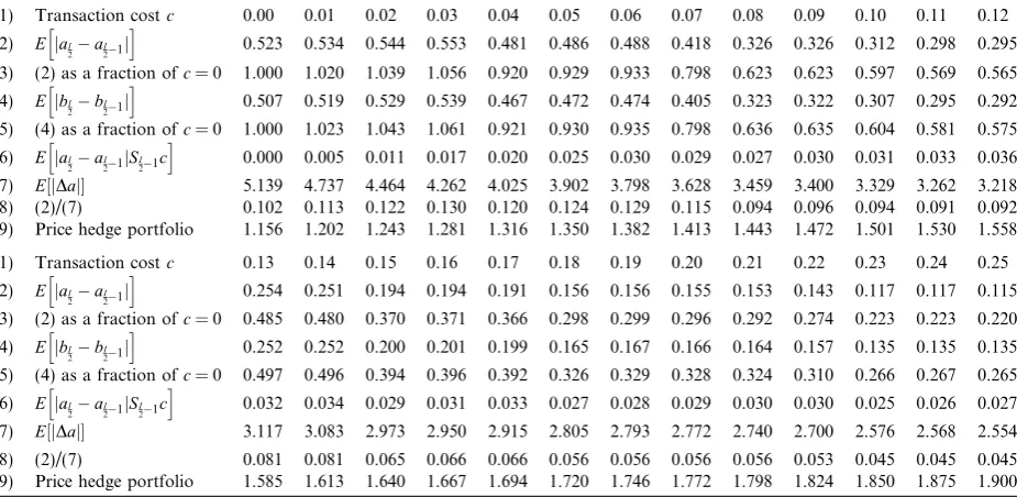
FromTable 1we see that the expected rebalanc-ing of the investment portfolio decreases when

increasing the proportional transaction cost (line 7). The major rebalancing from period one to two is also expected to decrease. However, it is not decreasing monotonically; for small transaction costs, there is actually an increase in the expected rebalancing (line 2). It is interesting to notice that for large transaction costs, the expected jump between period one and two is significantly smaller, as a fraction of the total expected rebalancing (line 8), than for lower transaction costs. This indicates that the hedge portfolio is constructed so as to reduce the expensive jump. For reasonable transac-tion costs for a life insurance company, say, less than 6%, the jump represents a greater fraction of the total expected rebalancing than for the case with zero transaction costs. For both c= 0.01,c= 0.02, 0

0.2 0.4 0.6 0.8 1 1.2 1.4

c = 0.00 c = 0.02 c = 0.10 c = 0.25 Value investment portfolio

Fig. 8. The number of units of the investment portfolio to include in the hedge portfolio for a given scenario for different levels of the proportional transaction costc.

0 0.2 0.4 0.6 0.8 1 1.2 1.4

c = 0.00 c = 0.02 c = 0.10 c = 0.25 Value investment portfolio

Fig. 9. The number of units of the risk free asset to include in the hedge portfolio for a given scenario for different levels of the proportional transaction costc.

and c= 0.03, the expected jump is in fact greater than for c= 0.00. This is somewhat surprising and may be an indication that transaction costs are not the most likely explanation for why insurance companies are not performing a major rebalancing of their investment portfolio at the end/beginning of each year.

4.4. More advanced price processes

Returns on financial assets in real world financial markets often have heavier tails than normally dis-tributed returns and volatilities are typically not

constant over time. Kozubowski and Rachev

(1994)find that the geometric stable distribution fits empirical returns well. This distribution typically has heavier tails than the normal distribution. There are also empirical evidence that volatilites follow stochastic processes (see e.g., Eraker et al., 2003) and that there are periods with high and low volatil-ities, often referred to as volatility clustering. Our analysis of the hedging strategy for the guarantee relies heavily on the assumed stochastic process for the investment portfolio. With more realistic price processes, e.g. exhibiting heavy tails and

vola-tility clustering, there are no generally accepted ways of discretizing the processes into scenario trees. One possible approach is to use Monte Carlo simulation, and subsequently construct a scenario tree as in Heitsch and Ro¨misch (2005). We leave the analysis of the hedging strategies using more advanced price processes for future research.

5. Conclusions

We have in this paper derived optimal hedging strategies for multi-period guarantees in the pres-ence of transaction costs. We found the cost of establishing the hedge portfolio to increase as trans-action costs increased. We also found the large rebalancing at the end of a period to decrease as a function of the transaction cost. Total rebalancing performed over the lifetime of the guarantee was also found to decrease when the transaction cost increases. However, for very small transaction cost, we actually found the total rebalancing to increase. This may be an indication that the presence of transaction costs does not explain, or is not the only explanation, for why life insurance companies are Table 1

(1) is the proportional transaction cost; (2) is the (risk neutral) expected rebalancing of the investment portfolio between period 1 and 2; (3) is (2) normalized withc= 0 as the basis; (4) is the (risk neutral) expected rebalancing of the risk free asset between period 1 and 2; (5) is (4) normalized withc= 0.6 is the expected cost of rebalancing between period 1 and 2; (7) is the expected total rebalancing of the investment portfolio; (8) is the expected rebalancing between period 1 and 2 as a fraction of the total rebalancing; (9) gives the (smallest) initial cost for the hedge portfolio

(1) Transaction costc 0.00 0.01 0.02 0.03 0.04 0.05 0.06 0.07 0.08 0.09 0.10 0.11 0.12

(2) E jaI

2a2I 1j

h i

0.523 0.534 0.544 0.553 0.481 0.486 0.488 0.418 0.326 0.326 0.312 0.298 0.295 (3) (2) as a fraction ofc= 0 1.000 1.020 1.039 1.056 0.920 0.929 0.933 0.798 0.623 0.623 0.597 0.569 0.565 (4) E jbI

2b2I 1j

h i

0.507 0.519 0.529 0.539 0.467 0.472 0.474 0.405 0.323 0.322 0.307 0.295 0.292 (5) (4) as a fraction ofc= 0 1.000 1.023 1.043 1.061 0.921 0.930 0.935 0.798 0.636 0.635 0.604 0.581 0.575 (6) E _jaI

2a

I

21jSI

21c

h i

0.000 0.005 0.011 0.017 0.020 0.025 0.030 0.029 0.027 0.030 0.031 0.033 0.036

(7) E½jDaj 5.139 4.737 4.464 4.262 4.025 3.902 3.798 3.628 3.459 3.400 3.329 3.262 3.218

(8) (2)/(7) 0.102 0.113 0.122 0.130 0.120 0.124 0.129 0.115 0.094 0.096 0.094 0.091 0.092

(9) Price hedge portfolio 1.156 1.202 1.243 1.281 1.316 1.350 1.382 1.413 1.443 1.472 1.501 1.530 1.558

(1) Transaction costc 0.13 0.14 0.15 0.16 0.17 0.18 0.19 0.20 0.21 0.22 0.23 0.24 0.25

(2) E _jaI

2a

I

21j

h i

0.254 0.251 0.194 0.194 0.191 0.156 0.156 0.155 0.153 0.143 0.117 0.117 0.115 (3) (2) as a fraction ofc= 0 0.485 0.480 0.370 0.371 0.366 0.298 0.299 0.296 0.292 0.274 0.223 0.223 0.220 (4) E jbI

2b2I 1j

h i

0.252 0.252 0.200 0.201 0.199 0.165 0.167 0.166 0.164 0.157 0.135 0.135 0.135 (5) (4) as a fraction ofc= 0 0.497 0.496 0.394 0.396 0.392 0.326 0.329 0.328 0.324 0.310 0.266 0.267 0.265 (6) E jaI

2a2I 1jSI21c

h i

0.032 0.034 0.029 0.031 0.033 0.027 0.028 0.029 0.030 0.030 0.025 0.026 0.027

(7) E_½jDa_j 3.117 3.083 2.973 2.950 2.915 2.805 2.793 2.772 2.740 2.700 2.576 2.568 2.554

(8) (2)/(7) 0.081 0.081 0.065 0.066 0.066 0.056 0.056 0.056 0.056 0.053 0.045 0.045 0.045

(9) Price hedge portfolio 1.585 1.613 1.640 1.667 1.694 1.720 1.746 1.772 1.798 1.824 1.850 1.875 1.900

S.-E. Fleten, S. Lindset / European Journal of Operational Research xxx (2006) xxx–xxx 9

not performing a major rebalancing of their invest-ment portfolio at the end of each year.

References

Black, F., Scholes, M., 1973. The Pricing of Options and Corporate Liabilities. Journal of Political Economy 81 (3), 637–654.

Boyle, P.P., Vorst, T., 1992. Option replication in discrete time with transaction costs. Journal of Finance 47 (1), 271–293. Cox, J.C., Ross, S.A., Rubinstein, M., 1979. Option pricing: a

simplified approach. Journal of Financial Economics 7, 229– 263.

Eraker, B., Johannes, M., Polson, N., 2003. The impact of jumps in volatility and returns. Journal of Finance 58 (3), 1269– 1300.

Heitsch, H., Ro¨misch, W., 2005. Scenario tree modelling for multistage stochastic programs, Preprint 296, DFG Research Center Matheon.

Kall, P., Wallace, S.W., 1994. Stochastic Programming. Wiley, Chichester.

Kozubowski, T.J., Rachev, S.T., 1994. The theory of geometric stable distributions and its use in modeling financial data. European Journal of Operations Research 74 (2), 310–324. Lindset, S., 2003. Discontinuous hedging strategies for

multi-period guarantees in life insurance. Journal of Risk Finance 5 (1), 51–63.

Miltersen, K., Persson, S.-A., 1999. Pricing rate of return guarantees in a Heath–Jarrow–Morton framework. Insur-ance: Mathematics and Economics 25 (3), 307–326. Soner, H.M., Shreve, S.E., Cvitanic, 1995. There is no nontrivial

hedging portfolio for option pricing with transaction costs. Annals of Applied Probability 5 (2), 327–355.