Stopping hot money

Munich Personal RePEc Archive

Stopping hot money

Reinhart, Carmen and Edison, Hali

University of Maryland, College Park, Department of Economics

December 2001

Stopping Hot Money Hali Edison

Board of Governors of the Federal Reserve Carmen M. Reinhart 1

University of Maryland and NBER

First draft: November 29, 1999

A revised version of this paper was published in:

Journal of Development Economics, Vol. 66 No. 2, December 2001, 533-553.

While high interest rates and foreign exchange sales are the most common way of dealing with a speculative attack in the foreign exchange market, several countries resorted to capital controls during recent periods of currency market turbulence. The purpose of this study is to use daily financial data to examine four of these capital controls episodes--Brazil, 1999, Malaysia 1998, Spain 1992, and Thailand 1997. We aim to assess the extent to which the capital controls were effective in delivering the outcomes that motivated their inception in the first place. We conclude that in two of the three cases (Brazil and Thailand), the controls did not deliver much of what was intended--although, one does not observe the counterfactual. By contrast, in the case of Malaysia the controls did align closely with the priors of what controls are intended to achieve: greater interest rate and exchange rate stability and more policy autonomy.

1 This paper was prepared for the National Bureau of Economic Research and

1 _{See Calvo, Leiderman, and Reinhart (1993) and Reinhart and Reinhart (1998).}

2

See Eichengreen (1994).

3_{See Edwards (1998) on this issue.}

I. Introduction

During the course of the 1990s, many emerging market economies experienced both the

highs and the lows of the international capital flow cycle. Early in the decade, many developing

countries regained access to international capital markets after many years of debt servicing

difficulties that gave them little recourse to new international lending. As capital began to find its

way back to countries in Asia and Latin America, the debate on how to manage a surge in capital

inflows emerged as one of the most pressing policy topics of the day. 1 _{Capital controls, when}

they were discussed at all, were examined in the context of liberalizing restrictions on capital

outflows or in terms of the relative merits of whether certain types of capital inflows--usually

short-term offshore borrowing--should be taxed or in any way restricted. Indeed, much of the

subsequent empirical work on capital controls was devoted to assessing whether these measures

were effective in achieving their stated objectives. For instance, Edwards (1998) examined

whether Chile’s reserve requirement policy bought its central bank some greater control over

short-term interest rates; Montiel and Reinhart (1999), looked at a panel of 15 emerging markets

(EMs) to determine whether these curbs or taxes on inflows were successful in influencing the

volume and composition of capital flows; and Cardoso and Goldfajn (1998) examined some of

these issues for the case of Brazil.

In the event, the EM capital flow surge proved to be as fragile and volatile in the 1990s as

it had been previously.2 _{The first prick of the capital flow bubble came with the Mexican crisis in}

4 _{See Kaminsky and Reinhart (1998).}

5_{See Bank of International Settlements (1999) for a detailed analysis of the events of the} fall of 1998.

mid-1997, much of emerging Asia was engulfed in a financial crisis of unprecedented severity for

that region.4 _{The Russian crisis and the near-bankruptcy of Long Term Capital Management}

(LTCM) in the fall of 1998 further dried up the remaining capital flows to EMs. 5 _{In early 1999,}

Brazil followed suit with a currency crisis of its own--raising (yet again) concerns about the

prospects for Argentina. Nor does this discussion provide an exhaustive chronology of recent

episodes of currency market turbulence. Colombia, which was one of the few Latin American

countries to avoid default in the early 1980s, fell into a severe financial crisis late in the summer of

1998 while Ecuador’s default on Brady and Eurobond obligations subsequently received much

attention from the financial press.

Given this string of disruptive events in international capital markets, it is not surprising

that the academic and policy discussion of and debate over capital controls began to shift

markedly in emphasis. The types of controls that were contemplated or used during several of the

recent crises were very different from the measures introduced during the inflow phase of the

capital flow cycle. Presumably this difference has a good theoretical grounding. As explained by

Bartolini and Drazen (1996), capital controls can convey information to the market about

policymakers’ preferences. No doubt policymakers would want to send different signals--which

are gotten from the controls--to slow the inflow of capital in good times relative to outflows in

bad times. The policies that were implemented to discourage capital inflows had two important

distinguishing features. First, the measures were typically introduced in a “tranquil” period during

6_{See Krugman (1998).}

7_{Indeed, institutional investors’ anxiety that a new wind was blowing regarding official} attitudes were heightened by the short-lived restrictions in Japan on short selling.

participants as being of a benign or “prudential” nature. Those measures very different from the

prototype capital control episode we examine in this paper, which were more akin to those

discussed in Paul Krugman’s policy advice appearing in the financial press in early 1998.6 _{In these}

writings, the emphasis was on the possible usefulness of capital controls as a means to buy time

during crisis periods. The policies, born out of necessity rather than precaution, are not typically

heralded as market-friendly. Malaysia’s controls in the fall of 1998 represented the most extreme

example of “adverse signaling”. Such signals were reenforced by Dr. Mahathir’s anti-foreigners

rhetoric at the time the controls were launched, which raised widespread concerns that even more

drastic measures, including expropriation, would follow.7

While high interest rates and foreign exchange sales are still the most common way of

dealing with a speculative attack in the foreign exchange market, several countries resorted to

introducing capital controls during recent periods of currency market turbulence. The purpose of

this study is to examine four of these crisis/capital controls episodes, three of them--Brazil, 1999,

Malaysia 1998, and Thailand 1997--in greater detail and Spain1992, serving as a comparison. We

aim to assess the extent to which the capital controls were effective and successful in delivering

some of the outcomes that motivated their inception in the first place.

The frequency of the data is daily. Except for Spain, which covers the 1991-1993 period,

the sample is 1995 through July 23, 1999. In addition to the four control episodes, there are two

“control group countries” the Philippines and South Korea, which had crises but did not introduce

market rates and changes in interest rates, equity market returns, exchange rate changes,

domestic-foreign interest rate differentials, bid-ask spreads on foreign exchange, onshore-offshore

interest rate spreads, and readings on the slope of the term structure of interest rates.

As to the empirical methodology, we employ an eclectic variety of tests: Tests for the

equality of moments and changes in persistence between capital control and no control periods;

principal component analysis--to assess contemporaneous comovement; block exogeneity tests in

a VAR framework to assess temporal international causality; GARCH tests for the effects of

controls on volatility--to assess changes in cross border volatility links, as in Edwards (1998) and;

Wald tests for structural breaks over a rolling window--to determine whether the timing of

structural breaks coincides with policy changes on capital controls.

There are, of course, several limitations and concerns with this kind of analysis. First,

results are episode specific because there are too few episodes to be confident in generating

“stylized facts.” Second, given that these kinds of controls are introduced during periods of

turbulence, it is particularly difficult to parse what owes to the controls from what is due to the

financial crisis per se. For instance, a generalized withdrawal from risk-taking (as what followed

the Russia/LTCM episode in the fall of 1998) could have similar implications and outcomes as the

introduction of capital controls. It is for that reason we examine some crises episodes for

countries that did not resort to controls as part of a control group.

With these caveats in mind, our key empirical findings are summarized below.

As to the behavior of the variables of interest in the control versus no-control period, we

find: Interest rates were less variable and usually more persistent following the introduction of

controls--but, except in Malaysia, domestic interest rates were not lower during the control

controls--especially so in the case of Thailand--consistent with the view that more of the burden of

adjustment falls on prices when the change in quantities is restricted. There is no evidence, except

for the case of Malaysia, that the controls were associated with more stable exchange rates.

Indeed, exchange rate variability increased significantly in all the other episodes.

As to the side-effects of capital controls, we find thatforeign exchange bid-ask spreads

were uniformly wider and more variable during the control periods. Of course, this was also the

case for the Philippines during its 1997 crisis--despite no new capital controls. Also,

onshore-offshore interest rate spreads widened and become more volatile following the introduction of

controls.

As to the central issue of insulating the economy from external shocks and gaining

greater policy autonomy, our results suggest that there is little evidence that capital controls

were effective in decoupling domestic interest rates from foreign interest rates--either

contemporaneously or temporally. The closest episode that meets this expectation is Malaysia.

There is also little evidence that these measures were effective in decoupling domestic exchange

rate changes from exchange rates abroad--either contemporaneously or temporally. Again,

Malaysia’s experience comes the closest to meeting this expectation. The evidence suggests that

equity markets continue to be internationally linked, despite the introduction of controls. Lastly,

financial crises appear to be a key determinant of the timing structural changes--more so than

capital controls.

The remainder of the paper is organized as follows. Section II discusses some of the

pertinent theoretical predictions as to what can be expected if the controls are effective. Section

III describes the measures and their chronology and presents the descriptive statistics for a variety

empirical tests performed and their outcomes and implications. The final section discusses

possible extensions and policy implications of the analysis.

II. Theoretical Predictions of the Effects of Controls

In this section, we first review some of the reasons most often voiced by policy makers for

resorting to capital controls during periods of turbulence. Knowing what the stated expectations

from the policy change are in the first place is essential to assess whether the policy was

“effective” or “successful.” Since many of these expectations are grounded on an implicit model,

we then proceed to summarize the implications of capital controls for some of the variables of

interest.

1. Reasons for resorting to capital controls during crises periods

The first line of defense by central banks dealing with speculative attacks on their

currencies is usually to sell off their holdings of foreign exchange. However, central bank

holdings of foreign exchange are often inadequate to support the currency and, even if the initial

stock is high by international standards, recurring runs on the currency can quickly deplete the

initial war chest. Not surprisingly, policy makers will often cite the need to stem the drain on

foreign exchange reserves as a motivation for introducing capital controls during periods of

extreme market stress.

Also central banks can (and often do) react to speculative pressures by raising interest rates,

occasionally to prohibitively high levels. However, given the consequences of high interest rates

on economic activity and debt servicing costs, this policy alternative is not particularly appealing

8 _{See Calvo and Reinhart (1999).}

9 _{Of course, imperfect asset substitutability and a time varying risk premia are sufficient to} explain a breakdown of uncovered interest parity--even in the absence of capital controls.

system is weak. Hence, capital controls are seen as a course of action which would enable the

monetary authorities to maintain lower (and more stable) interest rates than would be the case

under free capital mobility--especially if credibility has been lost. More generally, controls can (if

they are effective) fulfill the authorities’ desire to regain autonomy in monetary policy--without

floating the exchange rate.

Since volatile international bond and equity portfolio flows are frequently viewed as a

destabilizing force in asset markets and, more generally, in the financial system, another reason

which is often cited for introducing controls is the desire to reduce the volatility in asset prices.

2. Theoretical priors

The Mundellian trinity suggests that fixed (or quasi fixed) exchange rates, independent

monetary policy, and perfect capital mobility cannot be achieved simultaneously. Capital controls

are a way of allowing the authorities to retain simultaneous control over the interest rate and the

exchange rate. Capital controls may be particularly appealing when the authorities are reluctant

to allow the exchange rate to float freely, which is the case in most EMs.8 _{Fear of floating may}

arise for a variety of reasons, including the dollarization of liabilities--but for the purposes at hand,

however, those reasons are not central to our analysis. The important point for our analysis is that

controls introduce a systematic wedge between domestic and foreign interest rates. As uncovered

interest rate parity breaks down, the domestic policy interest rate (from the vantage point of a

wedge can be introduced by the authorities to influence the exchange rate systematically. One

example of this is the theoretical model of Reinhart and Reinhart (1998), who trace out the effects

of one of the simplest forms of capital controls--a reserve requirement. Depending on the degree

of competition among financial intermediaries, Reinhart and Reinhart show that the wedge

between foreign and domestic interest rates induced by the reserve requirement influences the

response of the exchange rate and the real economy to shocks.

The potential consequences of capital controls become even more persuasive in models

that provide an important role for asset stocks in affecting an economy. The general mechanism

at work is that, if the flow of capital is restricted in any way, then the burden of adjustment in

asset markets falls more on prices. Calvo and Rodriguez (1978) forst showed how sluggishness

in the flow of international assets can generate overshooting of the exchange rate. Reinhart (1998)

broadened that model by incorporating equity prices and introducing three different kinds of

restrictions on capital flows. The implication in Reinhart’s framework is that equity price

volatility should increase with the imposition of controls. The generic features of such models are

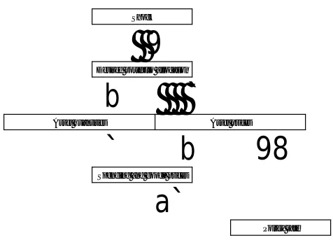
laid out in Figure 1. A shock to the desired portfolio allocation generally triggers adjustments to

both asset quantities and prices. Capital controls shift more of that adjustment toward prices and,

to the extent that they introduce interest rate wedges, may also alter the relationship between

asset prices and the policy rate.

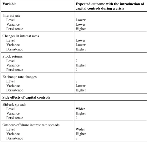
Table 1 provides a summary of the predictions of theory for selected financial variables.

Capital controls also have well defined predictions for central bank foreign exchange reserve

losses and capital outflows. Such data, however, is only available at lower frequencies and we

confine our emphasis here to financial indicators which are observable on a daily basis.

10 _{A recent example of evidence of monetary authorities’ concern with asset prices was} provided by the Hong Kong Monetary Authorities large-scale intervention in the equity market in the turbulent fall of 1998.

Less contemporaneous movement with international variables--particularly in interest rates and

exchange rates; a weaker causal (temporal) influence from foreign variables to domestic ones; a

decline in volatility spillovers; and evidence of structural breaks around the introduction of

controls.

The implications of a decline in market liquidity--whether owing to a capital control or a

generalized withdrawal from risk taking-- are also straightforward. Bid-ask spreads in the

market(s) where liquidity has diminished should widen and become more volatile.

A general caveat is in order, however. As the flow chart shown in Figure 1 highlights, if

asset prices are affected by the controls (as expected) and the policy interest rate responds to

asset prices, in turn, then controls may not be the insulating mechanism that they were intended to

Figure 1. Flowchart of a Generic Model

Shock

₉

Desired portfolio allocation

b

`

Asset quantities Asset prices

`

b

98

Spending and goods prices

a`

Policy rate

III. The Control Episodes

In this section, we describe the timing and nature of the selected capital control episodes

as well as some of the more relevant events surrounding the introduction and lifting of these

measures. We then confront the theoretical predictions with the data from four recent episodes.

1. The policy measures and chronology of events

The capital control episodes that we analyze are: Thailand (May 14, 1997-January 30,

three are recent examples of EM countries resorting to capital controls during periods of market

stress. We also examine, in less detail Spain (September 21- November 23, 1992), which was one

of the European countries to introduce controls during the Exchange Rate Mechanism (ERM)

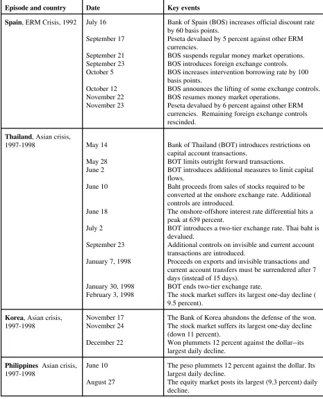
crisis of 1992-1993. The chronology of the episodes and further details of the measures are

summarized in Table 2.

In the case of Brazil, it is worth pointing out that the division between the “control” and

“no-control” period is somewhat blurred by the variety of measures Brazil introduced since the

mid-1990s measures that were along the lines of a Tobin tax on bond and equity purchases. As

the tax is paid upon the purchase of the asset, it disproportionally falls on investors which have a

very short holding period. Those measures were intended to curb what were perceived to be very

volatile portfolio capital inflows. By contrast, the measures announced on February 11 were

designed to force investment funds to hold more domestic government bonds--which lowered the

amount of other countries’ debt these fund could hold--thus restricting capital outflows.

As to the two control group countries, the Philippines and South Korea, the crisis episode

is set to span from the devaluation of the Thai baht on July 2, 1997 to end-July 1998, as these

countries were little affected by the Russian devaluation and the LTCM episode in the fall of

1998.

2. Methodology issues and limitations of the analysis

There are, of course, several limitations and concerns with the kind of analysis we

undertake. First, results are episode specific--not “stylized facts.” There are too few episodes for

that label. Second, given that these kinds of controls are introduced during periods of turbulence,

it is particularly difficult to separate what owes to the controls and what is due to the financial

Russia/LTCM episode in the fall of 1998) can have similar implications and outcomes as the

introduction of capital controls. Namely, international flows dry up, spreads widen volatility in

asset markets increases, and so on. Hence, the importance of having some crises episodes for

countries that did not resort to controls as part of a control group. Third, our empirical

methodology assumes linearities in relationships, which may break down during period of extreme

market stress--an issue that is highlighted in multiple-equilibria crises models.

3. Interest rates, stock returns and exchange rates during control and crises periods

In the preceding section, we provided a sketch of what theory predicts as regards the

behavior of selected key financial variables following the introduction of measures that curtail

international capital movements. In this section, we confront those predictions with the data from

four recent episodes. We examine the behavior of daily interest rates and changes in interest

rates, stock returns, exchange rate changes, bid-ask spreads on foreign exchange,

domestic-foreign interest rate differentials, and onshore-offshore interest rate differentials (where relevant).

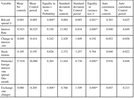
For each of these time series we provide descriptive statistics (mean and standard errors)

and test for the equality of first and second moments between the capital control and free capital

mobility periods. A correlogram for the individual subperiods is also used to assess whether the

persistence of shocks changes as a result of the change in policy. We also analyze this battery of

statistics and tests for two countries that had currency crises but did not impose controls. We

compare the crisis and tranquil periods with the aim of assessing the extent to which observed

changes in the key variables may be attributed to the crisis rather that the capital controls. Tables

3-8 report the results for each of the six countries.

there are any) align loosely with the theoretical predictions. While interest variability declines

following the introduction of controls, the reduction in interest rates is not significant; stock

market price volatility increases--but, again, the increase is not significant. Exchange rate

volatility increases markedly in the control period, as the “quasi-fixed” exchange rate regime was

abandoned shortly before the introduction of controls. Reflecting reduced market liquidity,

bid-ask spreads on foreign exchange widen and become more volatile after March 1, 1999.

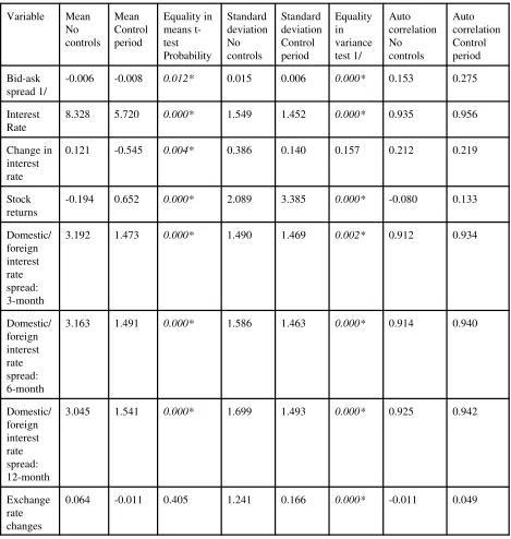
By contrast, Malaysia’s controls seem to be associated with the kind of changes one

would expect a priori if the controls were effective. The policy interest rate declines, and its level

becomes more stable and persistent. Similarly, the exchange rate also becomes more stable (the

ringgit was pegged to the US dollar on September 2, 1998). However, as the burden of

adjustment in asset markets falls more on prices than on quantities, equity prices become more

volatile. Indeed, as shown in Table 2, six days after the controls are introduced the stock market

suffered its largest one-day decline (a staggering 22 percent). As in the case of Brazil, reduced

market liquidity leads to wider and more volatile bid-ask spreads in the foreign exchange market.

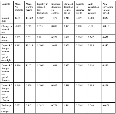
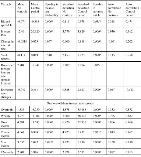
The pre- and post-control comparisons for Spain and Thailand look more like those for

Brazil rather than Malaysia’s. Interest rate variability declines--but interest rates actually increase

in both cases. However, domestic-foreign interest rate spreads actually decline and become more

stable for Spain. Yet, exchange rate variability increases (rather than declines), as Spain

ultimately devalued the peseta against other ERM currencies on October 12, 1992 and Thailand

floated the baht on July 2, 1997. As predicted by theory, equity prices are significantly more

volatile during the control period, and bid-ask spreads widen and become more volatile in both

countries. Thai onshore-offshore interest rate spreads widen significantly and become more

11_{These are unchanged for South Korea.}

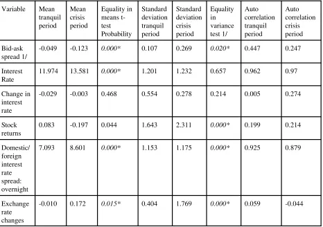
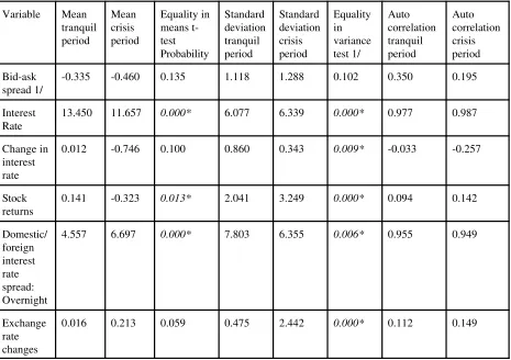
However, it will be difficult to trace to what extent some of these effects are owing

exclusively to the introduction of capital controls. While it is the case that for, the Philippines

and South Korea, interest rate variability does not decline during the crisis period (indeed, they

actually increase in Korea), equity price volatility is higher in both cases as the crisis unfolds. It is

also the case that, for the Philippines, market liquidity appears to deteriorate during the crisis as

bid-ask spreads on foreign exchange widen and become more variable.11

A summary of the main results is provided in Table 9. As to the behavior of the variables

of interest in the control versus no-control period, we find that: Interest rates were less variable

and usually more persistent following the introduction of controls--but, except in Malaysia,

interest rates were not lower during the control period. Stock returns tended to be more variable

following the introduction of capital controls--especially so in the case of Thailand--consistent

with the view that more of the burden of adjustment falls on prices when the change in quantities

is restricted. There is no evidence, except for the case of Malaysia, that the controls were

associated with more stable exchange rates. Indeed, exchange rate variability increased

significantly in all the other episodes.

IV. Are Control Periods Different?

In this section, we employ an eclectic variety of tests to examine whether the periods when

capital controls are in place are different. Specifically, we turn our attention to the issue of

external shocks, cross-border interdependence, and volatility spillovers. We employ principal

framework--to assess temporal international causality; GARCH tests for the effects of controls on

volatility spillovers--to assess changes in cross border volatility links, as in Edwards (1998) and;

Wald tests for structural breaks over a rolling window--to determine whether the timing of

structural breaks coincides with policy changes on capital controls.

1. Principal component analysis

To assess whether the degree of comovement across countries in several financial

variables is influenced by the introduction of capital controls, we applied principal component

analysis to the financial time series data over the control period and contrasted those results to the

subsample with no controls. A priori, one should expect a lower degree of comovement for the

country that has imposed controls during the period in which these are in place.

We focus on three daily time series, the domestic policy interest rate (described for each

country in Tables 3-9) the return on equity, and the change in the exchange rate (in percent) for

the five EM countries in our sample, Brazil, Malaysia, the Philippines, South Korea, and Thailand.

From these series, we constructed a smaller set of series, the principal components, that explain as

much of the variance of the original series as possible. The higher the degree of co-movement in

the original series, the fewer the number of principal components needed to explain a large

portion of the variance of the original series. In case where the original series are identical

(perfectly collinear), the first principal component would explain 100 percent of the variation in

the original series. Alternatively, if the series are orthogonal to one another, it would take as

many principal components as there are series to explain all the variance in the original series. In

that case, no advantage would be gained by looking at common factors, as none exist.

Ó

_'

P

_Ë

_P

and a unit standard deviation. This standardization ensures that all series receive uniform

treatment and the construction of the principal component indices is not influenced

disproportionately by the series exhibiting the largest variation. The correlation matrix of the

standardized series, Ó, is decomposed into its vectors (P) and the diagonal matrix of

Eigen-values (Ë).

The Eigen-vectors are the loading factors, or weights, attached to each of the original series.

For a particular time-series, the higher the degree of comovement with other series the higher (in

absolute value) its loading factor. If a particular time series is uncorrelated with the remaining

series included in the analysis, then its loading factor in the first principal component should be

close to zero. A priori, this is what we should expect to see for the time series for the country

with capital controls during the period in which these are in place.

In Table 9, we present the results for the various sample periods for interest rates. As

with the descriptive statistics presented in Tables 3-8, we also include the results for the two

control group countries, the Philippines and South Korea. In none of the capital control episodes

do the loading factors approach zero. In the case of Brazilian interest rates the loading factor

increases (in absolute terms), as Brazil and South Korea co-move inversely with the remaining

three countries. Malaysia’s interest rates, after its introduction of controls on September 1, 1998

continues to exhibit a high degree of comovement with neighboring Thailand and the Philippines.

While Thailand’s loading factor drops from 0.929 to 0.739 with the introduction of controls, it

12_{Thailand continues to show a high degree of comovement in the May 14, 1997-January} 30, 1998 period with Malaysia, the Philippines, and South Korea.

Table 10 summarizes the comparable results for stock returns. The extent of

contemporaneous co-movement of equity returns drops markedly for both Brazil (from

pre-control level of 0.328 to 0.171) and Malaysia (from 0.739 to 0.346) following the introduction of

controls and moderately so for Thailand.12 _{The clearest cut results, however, come from}

performing this exercise using daily exchange rate changes, as shown in Table 14. In both the

case of Brazil after capital controls are introduced on March 1, 1999 and following Malaysia’s

imposition of controls on September 1, 1998, their respective loading factors drop to almost zero

while the controls are in place suggesting that, at least contemporaneously, their exchange rate

changes are independent from exchange rate shocks elsewhere.

However, this analysis only provides a partial picture of what can be a fuller dynamic

cross-border interdependence. While principal component analysis reveals the extent to which

there is contemporaneous comovement across the countries in our study in interest rates, stock

returns and changes in the exchange rate across the various subsamples, interdependence may

have a temporal dimension as well. That is, a shock in one country may not have an immediate

effect on a second country but the effects of the shock may be spread out over the course of

several days. Given that our data is daily, such temporal relationships may be of greater

importance than for lower frequency data, where the synchronicity of financial market hours

across different regions and other institutional aspects of trading are less important. We turn to

this issue next.

r

_'

á

_%

A

(

L

)

r

_%

A

(

L

)

r

_%

A

(

L

)

r

_%

A

(

L

)

r

_%

A

(

L

)

r

_%

å

.

causal links among five of the countries following the introduction of capital controls, we proceed

much as we in the previous exercises. For Thailand, though, we now divide the sample into three

subperiods, the period preceding the controls which runs from January 1, 1995 to May 13, 1997,

the control period, which spans May 14, 1997 to January 30 and the post-control period which

ends on July 29, 1999. Similarly, for the Philippines and South Korea, we break up the sample

into the pre- and post-financial crisis and the crisis period, which as noted earlier spans July 2,

1997 through July 31, 1998. The focus is on cross-country links in interest rates, stock returns,

and changes in the exchange rate. A priori, if the controls are insulating the country from external

shocks and facilitating independent monetary policy, one should see a weakening in any

pre-existing causal links.

We employ a simple vector autoregression (VAR) framework that treats all variables as

potentially endogenous and include ten lags of each of the variables in the system. Omitting time

subscripts, a representative equation for domestic interest rates in Brazil (denoted by the subscript

b) in this five-equation system is given by,

The subscripts m, p, sk, and t refer to Malaysia, the Philippines, South Korea, and Thailand,

respectively. The lag operators are the A’s and å’s denote the random shocks. Because the

variance of the underlying fundamentals tends to increase during periods of turbulence, it is

13 _{See Rigobón (1998).}

system.13 _{Hubert/White robust standard errors were computed. The comparable system was}

estimated for daily stock returns and changes in the exchange rate (in percent). For each block of

regressors, we conducted F- and log-likelihood ratio tests that tested the null hypothesis of no

causal relationship.

Table 12 reports the results for interest rates; the detailed test statistics and their

associated probability values are presented in Appendix Tables 1-2. The columns “cause” the

rows; an N denotes that the null hypothesis of no causality was not rejected while a Y indicates

rejection of the null hypothesis at a 10 percent level of significance or higher. For example, the

top row, which summarizes the results for Brazil for the January 1, 1995-February 28, 1999

period shows four N entries, indicating that interest rates in the four remaining countries in the

system had no systematic influence on Brazilian interest rates prior to the introduction of controls.

The last column of Table 12 tallies the number of significant entries. Tables 13 and 14 summarize

in comparable manner the results for the daily stock returns and exchange rate changes.

Table 12 presents no evidence to indicate that in the cases of Brazil, Malaysia, and

Thailand capital controls weakened the international interdependence of interest rates--indeed,

quite the contrary. Prior to March 1, 1999, interest rates in Brazil were not influenced by interest

rate changes in the other four countries. In the more recent control period, however, interest

rates are significantly influenced by Korean and Thai rates. In the case of the Thai controls, a

similar tendency toward greater interdependence during the period during which the controls were

in place is also evident. For Malaysia, there is also no evidence of a decline in interdependence

but rather a shift in which country’s rates are significant. At a more general level, there is a

includes the pre-Asian crisis period, most of the regressors (other than lags of the dependent

variable) are not statistically significant at standard confidence levels. The more recent period

(i.e., post crisis) is quite different in that regard with a greater degree of interdependence among

the countries--particularly for the countries that did not introduce controls. Philippine and South

Korean interest rates are significantly influenced by interest rates in the remaining countries in the

sample.

Turning to stock returns, Table 13, presents several parallels to the results for interest

rates. In the case of Brazil, stock market interdependence is greater during the more recent

control period (South Korean and Thai stock returns are both statistically significant), while for

Thailand, the introduction of controls did not alter pre-existing causal relationships. The more

marked change is in Malaysia, where the number of countries whose equity market shocks have a

significant on the Malay market drops from three to one, as shown in the last column of Table 13.

This is a contrast to South Korea, where international interdependence in equity returns seems to

be on the rise during the more recent post-crisis period.

As regard daily exchange rate changes, Brazil’s exchange rate is influenced more

prominently by foreign exchange rate shocks during the capital control period. This result is not

surprising in light of the fact that the real was predetermined and confined to a narrow band

during most of the pre-control sample and allowed to fluctuate more freely during the control

period. The same observation applies to Thailand, which has continued with a managed float up

until the present time. As with equity returns, the importance of external exchange rate shocks

diminishes for Malaysia during the capital control period.

Taken together, these results suggest that capital controls had little effect in reducing

and Thailand. By contrast, Malaysia’s equity market and exchange rate are more autonomously

determined, following the introduction of controls. The results also suggest that interdependence

among four of the five EM economies (the exception is Malaysia) has increased in the wake of the

Asian financial crisis in the more recent period. Given that trade and financial linkages have not

changed markedly during this recent period, one interpretation for this greater interdependence is

that in the aftermath of the crisis financial market participants are more likely to lump these

economies into one group than they did previously.

3. Volatility and capital controls

While principal component analysis sheds light on contemporaneous international links and

the VARs added a temporal dimension to the analysis of international interdependence, both of

these approaches have focused on first moments. Yet, the descriptive statistics discussed in

Section III clearly suggested that there were important differences across regimes in second

moments (i.e., variances) in a high share of the financial variables analyzed. Furthermore, our

theoretical priors suggested that there should be such differences. In this subsection, we focus on

how capital controls and crises affect the volatility of interest rates and stock returns.

A related issue was recently examined in Edwards (1998). Using weekly interest rate data

for Argentina, Chile, and Mexico, Edwards (1998) analyzed the consequences of the Mexican

crisis for interest rate volatility in Argentina and Chile. The “Mexican spillover” dummies were

statistically significant for Argentina, irrespective of the specification used, and uniformly

insignificant for Chile. One possible interpretation of these results, he concluded, is that Chile’s

capital controls were effective in insulating Chile from the turmoil abroad.

14 _{In all cases a GARCH (1, 1) model was estimated.}

r

_'

_j

t&k t't&i

â

r

_%

_j

4

j'1

ã

r

jt

%

å

ó

rt

'

ù

%

dummy

%

áå

%

äó

(3)

Ä

r

_'

_j

t&k t_'t_&i

â

Ä

r

_%

_j

4

j_'1

ã

Ä

r

jt

%

å

ó

Ärt

'

ù

%

dummy

%

áå

%

äó

.

(4) heteroskedasticity (GARCH) models to examine whether was an observed change in volatility

during the capital controls episodes.14 _{As before, we will contrast these results to the crises}

episodes in the Philippines and South Korea where no controls are imposed during the crisis. We

consider the following models:

and

where the domestic nominal interest rate is denoted by r_t, in equation (3), the foreign interest rates

for the other four countries in the study are denoted by the r*_jt, and the random shock is denoted

by å. In the variance equation, ù is the mean of the variance; the lag of the mean squared residual

from the mean equation (i.e., å2

t-1 ) is the ARCH term and last period’s forecast variance (i.e., ó2

t-1) is the GARCH term. The term dummycis a dummy variable that takes on the value of one

during the control period for Brazil, Malaysia, and Thailand and zero otherwise. For the

The number of autoregressive lags, k, is reported for the cases k=0, 5, and 10. We also estimate

the model in first differences (Är_t,shown in equation 4) and for the case where the rs and r*_{s refer}

to equity returns. As discussed earlier, periods of turbulence that are part of our sample of daily

observations render the assumption of identically and independently distributed conditionally

normal disturbances in the basic GARCH model inadequate. Given the presence of

heteroskedastic disturbances in our sample, we use the methods described in Bollersev and

Woolridge (1992) to compute the Quasi-Maximum Likelihood covariances and standard errors.

The results for interest rates, changes in interest rates, and stock returns, are reported in

Tables 16-21. As to the specification for nominal interest rates, while both ARCH and GARCH

terms are statistically significant in Brazil, Malaysia, and Thailand (Table 16), the capital control

dummy variable is only significant for Malaysia--although this result is not robust across

alternative lag specifications. In the case of Malaysia, the controls dummy variable has the

anticipated negative sign, while in the case of Brazil and Thailand the sign is positive, although

not statistically significant. For the two countries that did not introduce capital controls (Table

17), the crisis dummy variable is not statistically significant.

Turning next to the results for the first differences of interest rates (shown in Tables 18

and 19), we find the same pattern. Among the three capital control and two crises without capital

controls episodes, the dummy variable is only significant for Malaysia for most of the lag profiles

used.

Finally, for daily equity price returns, the control dummy is significant and positive for

Thailand, indicating the control period was associated with above-average volatility in the equity

market (Table 20). However, it is difficult to attribute the increased volatility exclusively to the

r

_'

_j

t&k t_'t_&i

â

r

_%

_j

4

j_'1

ã

r

jt

%

å

.

capital account restrictions) was also associated with higher equity market volatility.

All in all, while the GARCH results do not point to across-the-board differences in

volatility across capital account regimes, the three cases where the control dummies are significant

(interest rates and interest rate changes in Malaysia and equity returns in Thailand) have the

expected sign.

4. The timing of structural breaks

The last of the tests that we perform involves an iterative search for breakpoints in interest

rate behavior over a rolling sample window. As before, the interest rate is modeled as a function

of its own lagged terms, contemporaneous interest rates in the other countries in the sample, and

a heteroskedastic disturbance,

The sample is broken into two subperiods, and we use a Wald test to test for the

restriction of the equality of coefficients in the two subperiods. The first of these tests breaks the

sample into January 1, 1995 through April 7, 1996 and a second 70-day sample period beginning

on April 8, 1996. The exercise is repeated recursively by moving the window by two days.

Hence, the number of observations in the early part of the subsample increases by two

observations with each iteration while the number of observations in latter part of sample remains

constant at 70 days over the rolling window. The Likelihood Ratio test identifies when the

15 _{Plots for the rolling probability values for each country for the entire sample are} available from the authors.

16 _{Indeed, a better way of analyzing these two episodes may be to also allow the early} subperiod to be a rolling 70 day window as well, rather than an ever-increasing sample beginning in 1995.

breaks are reported 15

None of these dates coincide exactly with the introduction of controls in Brazil and

Malaysia. For these two countries, evidence of structural breaks in the behavior of interest rates

come earlier. In the case of Brazil, the first break occurs on October 6, 1997, which is at the

height of the Asian crisis as Korea gets dragged down by the turmoil. Two other breaks occur in

1998, which are more difficult to associate with key international events. In the case of Malaysia,

the breakpoints run from June 24, 1997 through January 28, 1998 encompassing the height of the

Asian crisis. In both the case of Malaysia where controls are introduced in the fall of 1998 and

Brazil where the controls are in early 1999, the Wald tests would be biased toward identifying

earlier breaks, as once the crises observations are incorporated in the earlier sample, it becomes

harder to reject the hypothesis of stability. 16 _{For the case of Thailand (as is the case for the}

Philippines and South Korea), the dates structural breaks are closely aligned with the height of the

Asian financial crisis, indicating in all cases that the effects of the crisis on interest rate behavior

may be at the heart of the breakdown in past relationships.

5. Summary of findings

While the emphasis of the previous section was on examining possible changes in the key

financial variables, much of this section has been devoted to examining cross-border financial links

from external shocks and gaining greater policy autonomy, our results suggest that: there is little

evidence that capital controls were effective in decoupling domestic interest rates from foreign

interest rates--either contemporaneously or temporally. The closest to meeting this expectation is

Malaysia. There is also little evidence that these measures were effective in decoupling domestic

exchange rate changes from those changes abroad--either contemporaneously or temporally.

Again, the closest to meeting this expectation is Malaysia. The evidence suggests that equity

markets continue to be internationally linked, despite the introduction of controls. Finally,

financial crises appear to be a key determinant of the timing structural changes--more so than

capital controls.

V. Final Remarks

We have examined some recent experiences with capital controls during periods of market

stress. In two of the three cases (Brazil and Thailand), the controls did not appear to deliver

much of what was intended. Although, of course, one does not observe the counterfactual. By

contrast, in the case of Malaysia, the controls did align more closely with the priors of what

controls are intended to achieve--namely, greater interest rate and exchange rate stability and

more policy autonomy.

Generalized policy lessons are not possible from such a scanty set of experiences. Yet it

would appear that a fruitful area for future research would be to investigate the effectiveness of

controls for a more comprehensive set of episodes as it relates to the development and

international integration of the financial sector. One could speculate that Brazil’s relatively

sophisticated financial markets, which are second in liquidity to Hong Kong among EMs, and

in Malaysia. If, indeed, it were to be the case that financial sector development plays a prominent

role in explaining when capital account restrictions have a bite, then the policy implications for

References

Bank of International Settlements, 1999. (Basle, Switzerland: Bank for International Settlements).

Bartolini, Leonardo, and Alan Drazen,

Bollersev, Tim, and Jeffrey M. Woolridge, (1992). “Quasi-Maximum Likelihood Estimation and Inference in Dynamic Models with Time Varying Covariances,” Econometric Reviews 11, 143-172.

Calvo, Guillermo A., Leonardo Leiderman, and Carmen M. Reinhart, 1993. “Capital Inflows to Latin America: The Role of External Factors,” IMF Staff Papers 40, (March).

Calvo, Guillermo A., and Carmen M. Reinhart, 1999. “Fear of Floating,” mimeograph. (College Park: University of Maryland).

Calvo, Guillermo A., and Carlos A. Rodriguez, 1979. “A Model of Exchange Rate Determination Under Currency Substitution and Rational Expectations,” Journal of Political Economy

85, (June): 617-625.

Cardoso, Eliana, and Ilan Goldfajn, 1998. IMF Staff Papers , (March).

Dooley, Michael, “A Survey of the Academic Literature on Controls over International Capital Transactions,” IMF Staff Papers

Dornbusch, Rudiger

Edwards, Sebastian, 1998. “Interest Rate Volatility, Contagion and Convergence: An Empirical Investigation of the Cases of Argentina, Chile, and Mexico

Eichengreen, Barry,. “Trends and Cycles in Foreign Lending,” in Siebert

Kaminsky, Graciela L. and Carmen M. Reinhart, 1998. “Financial Crises in Asia and Latin America: Then and Now,” American Economic Review (May).

Mathieson, Donald, and Liliana Rojas-Suarez, IMF Occasional Paper, (Washington DC: International Monetary Fund).

Montiel, Peter, and Carmen M. Reinhart, 1999. “Do Capital Controls and Macroeconomic Policies Influence the Volume and Composition of Capital Flows? Evidence from the 1990s,” Journal of International Money and Finance (August).

Reinhart, Carmen M., and Vincent R. Reinhart, 1998 “Some Lessons for policy Makers On the Mixed Blessing of Dealing with Capital Inflows,” in M. Kahler, Financial Crises, (Cornell University Press).

Table 1. Selected Theoretical Predictions of the Effects of Capital Controls

Variable Expected outcome with the introduction of capital controls during a crisis

Interest rate Level Variance Persistence

Lower Lower Higher

Changes in interest rates Level

Variance Persistence

Lower Lower Higher

Stock returns Level Variance Persistence

? Higher ?

Exchange rate changes Level

Variance Persistence

? Lower Higher

Side effects of capital controls

Bid-ask spreads Level

Variance Persistence

Wider Higher ?

Onshore-offshore interest rate spreads Level

Variance Persistence

Table 2. A Chronology of Key Events

Episode and country Date Key events

Spain, ERM Crisis, 1992 July 16

September 17 September 21 September 23 October 5 October 12 November 22 November 23

Bank of Spain (BOS) increases official discount rate by 60 basis points.

Peseta devalued by 5 percent against other ERM currencies.

BOS suspends regular money market operations. BOS introduces foreign exchange controls. BOS increases intervention borrowing rate by 100 basis points.

BOS announces the lifting of some exchange controls. BOS resumes money market operations.

Peseta devalued by 6 percent against other ERM currencies. Remaining foreign exchange controls rescinded.

Thailand, Asian crisis,

1997-1998 May 14

May 28 June 2 June 10 June 18 July 2 September 23

January 7, 1998

January 30, 1998 February 3, 1998

Bank of Thailand (BOT) introduces restrictions on capital account transactions.

BOT limits outright forward transactions.

BOT introduces additional measures to limit capital flows.

Baht proceeds from sales of stocks required to be converted at the onshore exchange rate. Additional controls are introduced.

The onshore-offshore interest rate differential hits a peak at 639 percent.

BOT introduces a two-tier exchange rate. Thai baht is devalued.

Additional controls on invisible and current account transactions are introduced.

Proceeds on exports and invisible transactions and current account transfers must be surrendered after 7 days (instead of 15 days).

BOT ends two-tier exchange rate.

The stock market suffers its largest one-day decline ( 9.5 percent).

Korea, Asian crisis,

1997-1998

November 17 November 24

December 22

The Bank of Korea abandons the defense of the won. The stock market suffers its largest one-day decline (down 11 percent).

Won plummets 12 percent against the dollar--its largest daily decline.

Philippines Asian crisis,

1997-1998

June 10

August 27

The peso plummets 12 percent against the dollar. Its largest daily decline.

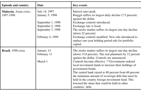
Table 2. A Chronology of Key Events (continued)

Episode and country Date Key events

Malaysia, Asian crisis,

1997-1998

July 14, 1997 January 5, 1998

September 1, 1998 September 2, 1998 September 7, 1998

February 4, 1999

Interest rates peak.

Ringgit suffers its largest daily decline (7.5 percent) against the dollar.

Exchange controls introduced. Exchange rate is fixed.

The stocks market suffers its largest one-day decline (down 22 percent).

Exchange controls modified. New rule introduced to replace one-year holding period rule for portfolio capital.

Brazil, 1999 crisis January 14

February 11

March 1

The stocks market suffers its largest one-day decline (down 15.8 percent). The real plummets by 12 percent against the dollar. Controls are announced.

Controls become effective. **Government ordered local investment funds to increase their holdings of government bonds.

Table 3. Brazil, January 1, 1995 to July 23, 1999: Descriptive Statistics for Daily Data

Variable Mean No controls

Mean Control period

Equality in means

t-test Probability

Standard deviation No controls

Standard deviation Control period

Equality in variance test 1/

Auto correlation

No controls

Auto correlation Control period

Bid-ask spread 1/

-0.001 -0.005 0.000* 0.004 0.005 0.001* 0.303 0.625 Interest

Rate

32.921 30.525 0.150 13.582 6.818 0.000* 0.940 0.849 Change in

interest rate

-0.049 -0.414 0.242 2.420 1.849 0.192 -0.052 -0.038

Stock returns

0.105 0.195 0.826 2.372 3.257 0.764 0.040 -0.022

Domestic/ foreign interest

rate spread: One-month

27.918 26.080 0.264 13.444 6.738 0.000* 0.916 0.848

Exchange rate changes

Table 4 Malaysia, January 1, 1995 to July 23, 1999: Descriptive Statistics for Daily Data Variable Mean No controls Mean Control period Equality in means t-test Probability Standard deviation No controls Standard deviation Control period Equality in variance test 1/ Auto correlation No controls Auto correlation Control period Bid-ask spread 1/

-0.006 -0.008 0.012* 0.015 0.006 0.000* 0.153 0.275 Interest

Rate

8.328 5.720 0.000* 1.549 1.452 0.000* 0.935 0.956 Change in

interest rate

0.121 -0.545 0.004* 0.386 0.140 0.157 0.212 0.219 Stock

returns

-0.194 0.652 0.000* 2.089 3.385 0.000* -0.080 0.133 Domestic/ foreign interest rate spread: 3-month

3.192 1.473 0.000* 1.490 1.469 0.002* 0.912 0.934

Domestic/ foreign interest rate spread: 6-month

3.163 1.491 0.000* 1.586 1.463 0.000* 0.914 0.940

Domestic/ foreign interest rate spread: 12-month

3.045 1.541 0.000* 1.699 1.493 0.000* 0.925 0.942

Exchange rate changes

Table 5. Spain, January 1, 1991 to December 31, 1993: Descriptive Statistics for Daily Data Variable Mean No controls Mean Control period Equality in means t-test Probability Standard deviation No controls Standard deviation Control period Equality in variance test 1/ Auto correlation No controls Auto correlation Control period Interest Rate

12.351 13.069 0.000* 1.379 0.218 0.009 0.988 0.832 Change in

interest rate

-0.009 0.012 0.075 0.088 0.093 0.188 -0.011 -0.016

Stock returns

0.062 0.065 0.981 0.978 1.488 0.000* 0.247 0.057 Domestic/ foreign interest rate spread: overnight

8.981 10.655 0.000* 3.681 0.651 0.000* 0.195 0.545

Domestic/ foreign interest rate spread: 3-month

8.496 11.071 0.000* 1.698 0.637 0.000* 0.914 0.857

Domestic/ foreign interest rate spread: 10-year

4.149 6.139 0.000* 0.907 0.589 0.000* 0.895 0.871

Exchange rate changes

Table 6. Thailand, January 1, 1995 to July 23, 1999: Descriptive Statistics for Daily Data Variable Mean No controls Mean Control period Equality in means t-test Probability Standard deviation No controls Standard deviation Control period Equality in variance test 1/ Auto correlation No controls Auto correlation Control period Bid-ask spread 1/

-0.074 -0.313 0.000* 0.111 0.978 0.033* 0.318 0.474 Interest

Rate

12.461 20.920 0.000* 5.779 3.829 0.000* 0.930 0.912 Change in

interest rate

-0.0318 0.073 0.067 0.600 0.818 0.000* -0.061 0.202 Stock

returns

-0.114 0.019 0.510 2.153 2.923 0.000* 0.115 0.258 Domestic/ foreign interest rate spread: 1-month

7.704 15.941 0.000* 5.609 3.804 0.075

Exchange rate changes

-0.047 0.361 0.000* 0.828 2.623 0.000* 0.047 -0.123

Onshore-offshore interest rate spreads

Overnight 1.336 16.730 0.000* 4.878 85.488 0.000* 0.332 0.872 Weekly 3.978 17.004 0.000* 7.900 58.323 0.000* 0.725 0.882

One-month

4.381 11.633 0.000* 6.420 22.955 0.000* 0.806 0.869

Three-month

4.067 6.988 0.000* 4.923 6.937 0.021* 0.845 0.867

Six-month

Table 7. Philippines, January 1, 1995 to July 23, 1999: Descriptive Statistics for Daily Data

Variable Mean tranquil period

Mean crisis period

Equality in means t-test Probability

Standard deviation tranquil period

Standard deviation crisis period

Equality in variance test 1/

Auto correlation tranquil period

Auto correlation crisis period

Bid-ask spread 1/

-0.049 -0.123 0.000* 0.107 0.269 0.020* 0.447 0.247 Interest

Rate

11.974 13.581 0.000* 1.201 1.232 0.657 0.962 0.97 Change in

interest rate

-0.029 -0.003 0.468 0.554 0.278 0.214 0.005 0.274

Stock returns

0.083 -0.197 0.044 1.643 2.311 0.000* 0.199 0.214 Domestic/

foreign interest rate spread: overnight

7.093 8.601 0.000* 1.153 1.175 0.000* 0.925 0.879

Exchange rate changes

Table 8. South Korea, January 1, 1995 to July 23, 1999: Descriptive Statistics for Daily Data

Variable Mean tranquil period

Mean crisis period

Equality in means t-test Probability

Standard deviation tranquil period

Standard deviation crisis period

Equality in variance test 1/

Auto correlation tranquil period

Auto correlation crisis period

Bid-ask spread 1/

-0.335 -0.460 0.135 1.118 1.288 0.102 0.350 0.195

Interest Rate

13.450 11.657 0.000* 6.077 6.339 0.000* 0.977 0.987 Change in

interest rate

0.012 -0.746 0.100 0.860 0.343 0.009* -0.033 -0.257 Stock

returns

0.141 -0.323 0.013* 2.041 3.249 0.000* 0.094 0.142 Domestic/

foreign interest rate spread: Overnight

4.557 6.697 0.000* 7.803 6.355 0.006* 0.955 0.949

Exchange rate changes

Table 9. Summary of Key Differences in Descriptive Statistics

Control period versus no-control period Crisis period versus tranquil

Variable Brazil Malaysia Spain Thailand Philippines South Korea

Bid-ask spread wider, more variable, more persistent wider, less variable, more persistent

wider wider, more variable, more persistent wider, more variable, less persistent no change Interest Rate

less variable lower, less variable, more persistent higher, less variable, less persistent higher, less variable

higher lower, more variable

Change in interest

rate

no change larger, less variable

no change more variable,

more persistent

no change less variable, more persistent

Stock returns

no change higher, more variable, more persistent more variable, less persistent more variable more variable lower, more variable Domestic/ foreign interest rate spread

less variable lower, less variable higher, less variable higher, less variable higher, more variable lower, less variable Exchange rate changes larger, more volatile and persistent smaller, less volatile larger, more variable larger, more variable larger, more variable, less persistent larger, more variable Onshore-offshore interest rate spread

n.a. n.a. n.a. wider, more variable, and more persistent

Table 10. Daily Interest Rates: Principal Component Analysis

Factor loadings in first principal component for:

Episode and time period R2 _{Brazil Malaysia Philippine}

s

South Korea

Thailand

Full sample 0.395 0.322 0.823 0.762 -0.456 0.867

Crises and capital control episodes

Brazil

Pre controls: January 1, 1995-February 28, 1999

0.359 0.312 0.833 0.801 -0.402 0.843

Controls: March 1, 1999-present

0.625 0.-654 0.712 0.912 -0.565 0.901

Malaysia

Pre controls: January 1, 1995-August 31, 1998

0.414 0.482 0.788 0.778 -0.571 0.827

Controls: September 1, 1998-present

0.700 -0.774 0.841 0.936 -0.696 0.928

Thailand

No controls: Remainder of sample

0.437 0.079 0.931 0.624 -0.686 0.929

Controls: May 14, 1997-January 30, 1998

0.533 0.773 0.624 0.828 -0.902 0.739

Crises episodes without capital controls

Philippinesand South Korea

Tranquil period: Remainder of sample

0.345 -0.848 0.527 0.081 0.646 0.727

Crisis: July 2, 1997-July 31, 1998

Table 11. Daily Stock Returns: Principal Component Analysis

Factor loadings in first principal component for:

Episode and time period R2 _{Brazil Malaysia Philippine}

s

South Korea

Thailand

Full sample 0.374 0.326 0.649 0.679 0.605 0.722

Crises and capital control episodes

Brazil

Pre controls: January 1, 1995-February 28, 1999

0.378 0.328 0.655 0.680 0.600 0.727

Controls: March 1, 1999-present

0.311 0.171 0.382 0.697 0.739 0.591

Malaysia

Pre controls: January 1, 1995-August 31, 1998

0.394 0.378 0.739 0.690 0.559 0.704

Controls: September 1, 1998-present

0.334 0.302 0.346 0.671 0.687 0.733

Thailand

No controls: Remainder of sample

0.363 0.302 0.591 0.677 0.598 0.746

Controls: May 14, 1997-January 30, 1998

0.403 0.377 0.742 0.709 0.570 0.705

Crises episodes without capital controls

Philippinesand South Korea

Tranquil period: Remainder of sample

0.330 0.270 0.518 0.667 0.611 0.699

Crisis: July 2, 1997-July 31, 1998

Table 13. Daily Exchange Rate Changes: Principal Component Analysis

Factor loadings in first principal component for:

Episode and time period R2 _{Brazil Malaysia Philippine}

s

South Korea

Thailand

Full sample 0.345 0.020 0.734 0.680 0.386 0.758

Crises and capital control episodes

Brazil

Pre controls: January 1, 1995-February 28, 1999

0.346 0.013 0.734 0.670 0.387 0.760

Controls: March 1, 1999-present

0.266 0.594 -0.000 0.472 -0.451 0.743

Malaysia

Pre controls: January 1, 1995-August 31, 1998

0.347 0.018 0.743 0.683 0.380 0.757

Controls: September 1, 1998-present

0.282 0.188 0.039 0.747 0.488 0.759

Thailand

No controls: Remainder of sample

0.380 0.044 0.814 0.711 0.207 0.828

Controls: May 14, 1997-January 30, 1998

0.328 0.109 0.694 0.671 0.406 0.728

Crises episodes without capital controls

Philippinesand South Korea

Tranquil period: Remainder of sample

0.272 0.261 0.560 0.737 0.378 0.543

Crisis: July 2, 1997-July 31, 1998

0.351 0.087 0.747 0.677 0.366 0.777

Table 13. Daily Interest Rates: Causality Tests Hubert/White Robust Standard Errors

Brazil Malaysia Philippine

s

South Korea

Thailand Numbe

r signifi-cant

Crises and capital control episodes

Brazil

Pre controls:

January 1, 1995-February 28, 1999

N N N N 0

Controls: March 1, 1999-present N N Y Y 2

Malaysia

Pre controls:

January 1, 1995-August 31, 1998

N N N Y 1

Controls: September 1, 1998-present Y N N N 1

Thailand

Pre controls:

January 1, 1995-May 13, 1997

N Y N N 1

Controls: May 14, 1997-January 30, 1998

N N Y Y 2

Post controls:

January 31, 1998-present

N N N Y 1

Crises episodes without capital controls

Philippines

Pre crisis:

January 1, 1995-July 1, 1997

N N N Y 1

Crisis: July 2, 1997-July 31, 1998 N N N N 0

Post crisis:

August 1, 1998-present

Y Y Y Y 4

South Korea

Pre crisis:

January 1, 1995-July 1, 1997

N N N N 0

Crisis: July 2, 1997-July 31, 1998 N Y N N 1

Post crisis:

August 1, 1998-present