Numerical Solution of Fourth Order Boundary Value Problems by Petrov Galerkin Method with Cubic B splines as basis Functions and Quintic B Splines as Weight Functions

(1)

Numerical Solution of Fourth Order Boundary Value

Problems by Petrov-Galerkin Method with Cubic

B-splines as basis Functions and Quintic B-Splines as

Weight Functions

K.N.S.Kasi Viswanadham

Department of Mathematics National Institute of Technology

Warangal – 506004 (INDIA)

S.M.Reddy

Department of Mathematics National Institute of Technology

Warangal – 506004 (INDIA)

ABSTRACT

This paper deals with a finite element method involving Petrov-Galerkin method with cubic B-splines as basis functions and quintic B-splines as weight functions to solve a general fourth order boundary value problem with a particular case of boundary conditions. The basis functions are redefined into a new set of basis functions which vanish on the boundary where the Dirichlet type of boundary conditions are prescribed. The weight functions are also redefined into a new set of weight functions which in number match with the number of redefined basis functions. The proposed method was applied to solve several examples of fourth order linear and nonlinear boundary value problems. The obtained numerical results were found to be in good agreement with the exact solutions available in the literature.

Keywords

Petrov-Galerkin method, Cubic B-spline, Quintic B-spline, Fourth order boundary value problem, Absolute error.

1. INTRODUCTION

In this paper, we consider a general fourth order linear boundary value problem

(4)

0 1 2 3

4

( ) ( ) ( ) ( ) ( ) ( ) ( ) ( ) ( ) ( ) ( ) ,

a x y x a x y x a x y x a x y x

a x y x b x c x d

  

  

   

(1)

subject to boundary conditions

0 0 1 1

( ) , ( ) , ( ) , ( )

y c A y d C y c A y d C (2) where A0, C0, A1, C1 are finite real constants and a0(x), a1(x),

a2(x), a3(x), a4(x) and b(x) are all continuous functions

defined on the interval [c, d].

The fourth order boundary value problems occur in a number of areas of applied mathematics, among which are fluid mechanics, elasticity and quantum mechanics as well as in science and engineering. The existence and uniqueness of the solution for these types of problems have been discussed in Agarwal [1]. Finding the analytical solutions of such type of boundary value problems in general is not possible. Over the years, many researchers have worked on boundary value problems by using different methods for numerical solutions [2-20]. So far various numerical methods such as Cubic spline

method [2], Iterative methods [3], Perturbed collocation method [4], Modified decomposition method [5], Decomposition method [6], Differential transform method [7, 8], A higher order B-spline collocation method [9], Homotopy perturbation method [10], Variational iteration technique [11], Sinc-Galerkin method [12], Spline techniques [13-16], Galerkin method with quintic B-splines [17], B-spline collocation method [18], Cubic B-spline collocation method [19], Galerkin method with cubic B-splines [20] have been employed to solve fourth order boundary balue problems. So far, fourth order boundary value problems have not been solved by using Petrov-Galerkin method with cubic B-splines as basis functions and quintic B-splines as weight functions . This motivated us to solve a fourth order boundary value problem by Pertrov-Galerkin method with cubic B-splines as basis functions and quintic B-splines as weight functions.

In this paper, the effort is made to present a simple finite element method which involves Petrov-Gelerkin approach with cubic B-splines as basis functions and quintic B-splines as weight functions to solve the fourth order boundary value problem of the type (1)-(2). This paper is organized as follows. Section 2, deals with the justification for using Galerkin Method, In Section 3, a description of Petrov-Galerkin method with cubic B-splines as basis functions and quintic B-splines as weight functions is explained. In particular we first introduce the concept of cubic B-splines, quintic B-splines and followed by the proposed method with the specified boundary conditions. In Section 4, the procedure to solve the nodal parameters has been presented. In section 5, the proposed method is tested on several linear and nonlinear boundary value problems. The solution to a nonlinear problem has been obtained as the limit of a sequence of solution of linear problems generated by the quasilinearization technique [21]. Finally, in the last section, the conclusions are presented.

2. JUSTIFICATION FOR USING

PETROV-GALERKIN METHOD

(2)

solution for a given differential equation exists and is unique under appropriate conditions [22,23] irrespective of properties of a given differential operator. Further, a weak solution also tends to a classical solution of given differential equation, provided sufficient attention is given to the boundary conditions[24]. That means the basis functions should vanish on the boundary where the Dirichlet type of boundary conditions are prescribed and also the number of weight functions should match with the number of basis functions. Hence in this paper the effort is made to use the Petrov-Galerkin method with cubic B-splines as basis functions and quintic B-splines as weight functions to approximate the solution of fourth order boundary value problem.

3. DESCRIPTION OF THE METHOD

Definition of cubic B-splines and quintic B-splines:

The cubic B-splines and quintic B-splines are defined in [25-27]. The existence of cubic spline interpolate s(x) to a function in a closed interval [c, d] for spaced knots (need not be evenly spaced) of a partition

d x x x

x

c ₀ ₁... _n_1 _n

is established by constructing it. The construction of s(x) is done with the help of the cubic B-splines. Introduce six additional knots x-3, x-2, x-1, xn+1, xn+2 and xn+3 in such a way

that

x-3<x-2<x-1<x0 and xn<xn+1<xn+2<xn+3.

Now the cubic B-splines

B

i

(

x

)'

s

are defined by

3 2 2 2 2

(

)

,

[

,

]

( )

0,

i r i i r i i r

x

B x

x

otherwise



     











_

 





where 3

3

(

) ,

(

)

0,

r r

r

x

if x

x

if x

x













_{ }





and 2 2

( )

(

)

i r r i

x





 







where {B-1(x), B0(x), B1(x),…, Bn-1(x), Bn(x), Bn+1(x)} forms a basis for the space

S

₃

( )



of cubic polynomial splines. Schoenberg [27] has proved that cubic B-splines are the unique nonzero splines of smallest compact support with the knots at

x-3<x-2<x-1<x0<x1<…<xn-1<xn<xn+1<xn+2<xn+3.

In a similar analogue quintic B-splines Ri(x)'s are defined by

5 3 3 3 3

(

)

,

[

,

]

( )

0,

i r i i r i i r

x

R x

x

otherwise



     



_



_



_

 





where and 3 3

( )

(

)

i r r i

x





 







where {R (x), R (x), R(x), R (x),…, R (x), R(x), R (x),

polynomial splines with the introduction of four more additional knots

x

₅

,

x

₄

,

x

n₄

,

x

n₅ to the already existing knots

x

_₃ to

x

_n₃. Schoenberg [27] has proved that quintic

B-splines are the unique nonzero splines of smallest compact support with the knots at

x-5<x-4<x-3<x-2<x-1<x0<x1<…

<xn-1<xn<xn+1<xn+2<xn+3<xn+4<xn+5.

To solve the boundary value problem (1) subject to boundary conditions (2) by the Petrov-Galerkin method with cubic B-splines as basis functions and quintic B-B-splines as weight functions, the approximation for y(x) is defined as

1 1

( )

n j j j

y x



B x









(3)

where



_j,

s

are the nodal parameters to be determined and

( ) '

j

B x s

are cubic B-spline basis functions. In Petrov-Galerkin method, the basis functions should vanish on the boundary where the Dirichlet type of boundary conditions are specified. In the set of cubic B-splines {B-1(x), B0(x), B1(x),…, Bn-1(x), Bn(x), Bn+1(x)}, the basis functions B-1(x), B0(x), B1(x),

Bn-1(x), Bn(x) and Bn+1(x) do not vanish at one of the boundary

points. So, there is a necessity of redefining the basis functions into a new set of basis functions which vanish on the boundary where the Dirichlet type of boundary conditions are specified. The procedure for redefining of the basis functions is as follows.

Using the definition of cubic B-splines and the Dirichlet boundary conditions of (2), the approximate solution at the boundary points can be written as

0 ( ) ( )0 1 1( )0 0 0( )0 1 1( )0

A y c y x 



_B_ x 



B x 



B x (4)

0 1 1

1 1

( )

(

)

(

)

(

)

(

)

n n n n n n n

n n n

C

y d

y x

B

x

B x

B

x



   





(5)

Eliminating



_₁ and



_n_₁from the equations (3), (4) and (5), we get 0

( )

n j j j

y x

w x



P x







(6)

where

0 0

1 1

1 0 1

( )

_n

(

_n

)

n

A

C

w x

B

x

B

x

B

_

x



B

_

x







(7)

0 1 1 0 1 1 ( )

( ) ( ) , 0,1

( )

( ) ( ) , 2, 3,..., 2

( )

( ) ( ) , 1,

( ) j j j j j n j n n n B x

B x B x j

B x

P x B x j n

B x

B x B x j n n

B x           _     _ _{ }  (8)

The new set of basis functions in the approximation y(x) is

(3)

approximation is n + 1, where as the number of weight functions is n+5. So, there is a need to redefine the weight functions into a new set of weight functions which in number match with the number of basis functions. The procedure for redefining the weight functions is as follows:

Let the approximation for y(x) be taken as

2 2

( )

n j j j

y x



R x









(9)

where

R x s

j

( ) '

are quintic B-splines and here we assume that

above approximation y(x) satisfies corresponding homogeneous boundary conditions of the given boundary conditions (2). That means y(x) defined in (9) satisfies the conditions

y c

( ) 0, ( ) 0, ( ) 0, ( ) 0



y d



y c





y d





(10)

Applying the boundary conditions (10) to (9), the approximate solution at the boundary points can be written as

2

0 0

2

( )

_j _j

( )

0

j

y c

y x



R x









(11)

2

( )

(

)

(

)

0

n

n j j n

j n

y d

y x



R x



 







(12)

2

0 0

2

( )

_j _j

( )

0

j

y c

y x



R x

















(13)

2

( )

(

)

(

)

0

n

n j j n

j n

y d

y x



R x



 















(14) Eliminating

2



_ ,

1



_ , _n_₁ and



_n_₂ from the equations (9) and (11) to (14), we get the approximation for y(x) as

0

( )

n j j j

y x



T x





(15)

where 0 1 1 0 1 1 ( )

( ) ( ) , 0,1, 2

( )

( ) ( ) , 3, 4,..., 3

( )

( ) ( ) , 2, 1,

( ) j j j j j n j n n n S x

S x S x j

S x

T x S x j n

S x

S x S x j n n n

S x          _       _  _ _{ } _    (16) 0 2 2 0 2 2 ( )

( ) ( ) , 1, 0 ,1, 2

( )

( ) ( ) , 3, 4,..., 3

( )

( ) ( ) , 2, 1, , 1

( ) j j j j j n j n n n R x

R x R x j

R x

S x R x j n

R x

R x R x j n n n n

R x            _     _ _{ } _ _  (17)

Now the new set of weight functions for the approximation y(x) is

{ ( ),

T x j

_j



0,1,..., }

n

. Here

T x

j

( )

's and their

derivatives vanish on the boundary.

Applying the Petrov-Galerkin method to (1) with the new set of basis functions { ( ),P x j_j 0,1,..., }n and with the new set of weight functions

{ ( ),

T x j

_j



0,1,..., }

n

, we get

0

(4)

0 1 2 3

4

( ) ( ) ( ) ( ) ( ) ( ) ( ) ( )

( ) ( ) ( ) ( ) ( ) for i 0, 1, , n.

[

]

n n x x x i i x

a x y x a x y x a x y x a x y x

a x y x

T

x dx b x T x dx

         



(18)

Integrating by parts the first three terms on the left hand side of (18) and after applying the boundary conditions prescribed in (2), we get









0 0 0 2 (4)

0 2 0 1

2

0 1 0

3 2 3 ( ) ( ) ( ) ( ) ( ) ( ) ( )

[

( ) ( )

]

( ) n n n x

i i x

x

i _x i

x d

a x T x y x dx a x T x C dx

d d

a x T x A a x T x y x dx

dx dx    



(19) 0 0 2

1

( ) ( )

( )

2

[

1

( ) ( )

]

( )

n n

x x

i i

x x

d

a x T x y

x dx

a x T x y x dx

dx









(20)

0 0

2( ) ( ) ( )

[

2( ) ( )

]

( )

n n x x i i x x d d

a x T x y x dx a x T y

x x x dx

   



(21)

Substituting (19), (20) and (21) in (18) and using the approximation for y(x) given in (6), and after rearranging the terms for resulting equations, we get system of equations in the matrix form as

A





B

(22)

where A[a_ij];

0 3 2 0 1 3 2 2 3 4

{[

[ ( ) ( )]

( ) ( )] ( )

( ) ( ) ( )}

n x

ij _x i i

i i j

i j

d

a

a x T x

dx

d

a x T x

a x T x P x

dx

a x T x P x dx















for i = 0, 1,…, n; j = 0, 1,…, n. (23)

[ ];

b

_i



B

0 0 3 0 3 2

1 2 3

2

4 2 0 1

2 0 1 2 { ( ) ( ) [ [ ( ) ( )] [ ( ) ( )] [ ( ) ( )] ( ) ( )] ( ) ( ) ( ) ( )} [ ( ) ( )] [ ( ) ( )] n n x

i _x i i

i i i

i i x

i x d

b b x T x a x T x

dx

d d

a x T x a x T x a x T x w x

dx dx

d

a x T x w x dx a x T x C dx

d

a x T x A dx         



for i = 0, 1, ..., n. (24) and

0 1

[

]

T

.

n

(4)

4. PROCEDURE TO FIND SOLUTION

FOR NODAL PARAMETERS

A typical integral element in the matrix

A

is

1

0 n

m m

I







where 1

( ) ( ) ( )

m m

x

m _x i j

I 



v xr x Z x dx and ( )r xj are the cubic

B-spline basis functions or their derivatives. ( )v xi are the quintic

B-spline weight functions or their derivatives. It may be noted that

I

_m



0

if

3 3 2 2 1

(x_i_,x_i_ )(x_j_ ,x_j_ )(x x_m, _m_) .

To evaluate each

I

_m, we employed 5-point Gauss-Legendre

quadrature formula. Thus the stiffness matrix

A

is a nine diagonal band matrix. The nodal parameter vector



has been obtained from the system A



B using the band matrix solution package. The boundary value problems (1) - (2) have been solved by the proposed method with the help of a computer program written in FORTRAN-90 code.

5. NUMERICAL RESULTS

To demonstrate the applicability of the proposed method for solving the fourth order boundary value problems of the type (1) and (2), we considered three linear and four nonlinear boundary value problems. The obtained numerical results for each problem are presented in tabular forms and compared with the exact solutions available in the literature.

Example 1: Consider the linear boundary value problem

y

(4)



4 y



1,

  

1 x

1

(25)

subject to

( 1)

(1)

0 y

 

y



,

sinh 2 sin 2

( 1)

,

4(cosh 2 cos 2)

y

  





sin 2 sinh 2

(1)

4(cosh 2 cos 2)

y

 





.

The exact solution for the above problem is

sinh1sin1sinh sin cosh1cos1cosh cos

.25 1 2 .

(cos 2 cosh 2)

x x x x

y _   _



 

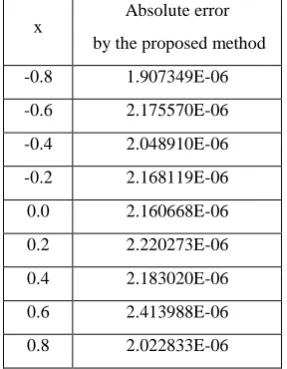
The proposed method is tested on this problem where the domain [-1, 1] is divided into 10 equal subintervals. The obtained numerical results for this problem are given in Table 1. The maximum absolute error obtained by the proposed method is 2.413988x10-6.

(4)

_{(8 7}

3

₎

x

_,

₀

₁

y



xy

  

x



x e

 

x

(26)

subject to

y

(0)



y

(1)



0,

y



(0) 1,



y

  

(1)

e

.

_y



_x

(1



_{x e}

) .

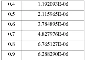
x

[image:4.595.357.501.89.274.2]

The proposed method is tested on this problem where the domain [0, 1] is divided into 10 equal subintervals. The obtained numerical results for this problem are given in Table 2. The maximum absolute error obtained by the proposed

Table 1: Numerical results for Example 1

x

Absolute error

by the proposed method

-0.8 1.907349E-06

-0.6 2.175570E-06

-0.4 2.048910E-06

-0.2 2.168119E-06

0.0 2.160668E-06

0.2 2.220273E-06

0.4 2.183020E-06

0.6 2.413988E-06

[image:4.595.358.501.308.492.2]

0.8 2.022833E-06

x

Absolute error

0.1 8.642673E-07

0.2 9.387732E-07

0.3 8.344650E-07

0.4 1.192093E-06

0.5 2.115965E-06

0.6 3.784895E-06

0.7 4.827976E-06

0.8 6.765127E-06

0.9 6.288290E-06

(4)

,

0

1 (

3)

x

y



 

y



e

x





x



(27) subject to

y

(0) 1,



y

(1)



0,

y



(0)



0,

y



(1)

 

e

.

The proposed method is tested on this problem where the domain [0, 1] is divided into 10 equal subintervals. The obtained numerical results for this problem are given in Table 3. The maximum absolute error obtained by the proposed method is 4.500151x10-6.

x Absolute error

0.1 8.642673E-07

(5)

0.4 1.192093E-06

0.5 2.115965E-06

0.6 3.784895E-06

0.7 4.827976E-06

0.8 6.765127E-06

0.9 6.288290E-06

Example 4: Consider the nonlinear boundary value problem

(4) 2 10 9 8 7 6 4

4 4 4 8 4 120 48,

0 1 (28)

y y x x x x x x x

x

        

 

subject to

y

(0)



0,

y

(1) 1,



y



(0)



0,

y



(1) 1.



The nonlinear boundary value problem (28) is converted into a sequence of linear boundary value problems generated by quasilinearization technique[21] as

(4) 10 9 8

( 1) ( ) ( 1)

7 6 4 2

( )

[2

]

4

8

4

120 48 [

] ,

n n n

n

y

x

y







 













n=0, 1, 2, … (29)

subject to

(n1)

(0)

0,

(n1)

(1) 1,

y

_



y

_



y₍_n_₁₎(0) 0, y₍_n_₁₎(1) 1.

[image:5.595.95.238.71.172.2]

Here y(n+1) is the(n1)th approximation for y(x). The domain [0, 1] is divided into 10 equal subintervals and the proposed method is applied to the sequence of linear problems (29). The obtained numerical results for this problem are presented in Table 4. The maximum absolute error obtained by the proposed method is 1.120567x10-5.

x Absolute error

0.1 3.879890E-06

0.2 1.497567E-06

0.3 2.533197E-06

0.4 5.781651E-06

0.5 8.285046E-06

0.6 9.894371E-06

0.7 1.037121E-05

0.8 1.120567E-05

0.9 9.357929E-06

 

2

2 (4)

,

0 in

1 s

x

sin

x

y







y



 

x

(30)

subject to y(0)=0, y(1)=sin1, y(0)1, y (1) cos1.

The exact solution for the above problem is ysin .x The nonlinear boundary value problem (30) is converted into a sequence of linear boundary value problems generated by quasilinearization technique [21] as

(4) 2 2

(n1) [2 ( )n ] (n 1) sin sin [ ( )n ] , 0,1, 2,...

y _  y y_  x x y n (31)

subject to y(n+1)(0)=0, y(n+1)(1)=sin1,

(n1)

(0) 1

y



_



,

(n1)(1) cos1. y_  Here

y

₍_n_₁₎ is the ( 1)th

n approximation for y(x). The domain [0, 1] is divided into 10 equal subintervals and the proposed method is applied to the sequence of linear problems (31). The obtained numerical results for this problem are presented in Table 5. The maximum absolute error obtained by the proposed method is 5.334616x10-6.

(4)

₆

4y

₁₂₍₁

_{) , 0}

4

₁

y



e



 



x



 

x

(32)

subject to

(0)

0,

(0) 1, (1)

ln 2,

(1)

0.5. y



y





y



y





The exact solution for the above problem is y=ln(1+x).

[image:5.595.96.239.502.689.2]

The nonlinear boundary value problem (32) is converted into a sequence of linear boundary value problems generated by quasilinearization technique [21] as

x Absolute error

0.1 6.929040E-07

0.2 2.041459E-06

0.3 3.606081E-06

0.4 4.947186E-06

0.5 5.334616E-06

0.6 4.947186E-06

0.7 4.172325E-06

0.8 2.801418E-06

0.9 1.132488E-06

( ) ( )

4 4

(4) 4

( 1) [24 ] ( 1) 12(1 ) [6 24 ( )],

n n

y y

n n n

y   e y    x e  y n = 0,1,2,… (33)

subject to

(n1)(0) 0, (n1)(0) 1, (n 1)(1) ln 2, (n 1)(1) 0.5. y _  y_  y _  y_  Here y(n+1) is the (n+1)

th

(6)

[image:6.595.359.501.71.174.2]

x

Absolute error

0.1 1.937151E-07

0.2 1.579523E-06

0.3 3.278255E-06

0.4 4.678965E-06

0.5 5.125999E-06

0.6 4.678965E-06

0.7 3.933907E-06

0.8 2.622604E-06

0.9 1.013279E-06

2 2

(4) 2

2 72(1 5 5 ) 2 6,

1 1 ( )

x x

y x x

     

  

0 < x < 1 (34)

subject to

(0)

0, (0)

0, (1)

0. y



y





y



y





The exact solution for the above problem is 3 3

(1 ) .

yx x The nonlinear boundary value problem (34) is converted into a sequence of linear boundary value problems generated by quasilinearization technique [21] as

2 2

( ) (4)

( 1) 2 2 ( 1) 2 6

( )

2 2 2

( ) 2

2 2 2

( ) ( )

2

(1 [ ] ) 1 ( )

2 [ ]

72(1 5 5 ) ,

(1 [ ] ) 1 [ ]

n

n n

n

n n

x y x

y y

y x x

x y x

x x

y y

  _   _{ }

    

 

n=0,1, 2, … (35)

subject to

(n1)(0) 0, (n1)(0) 0, (n1)(1) 0, (n1)(1) 0 y _  y_  y _  y_ 

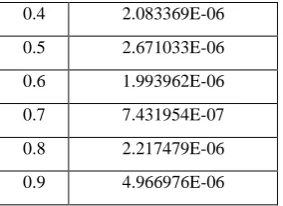
[image:6.595.96.238.90.272.2]

Here y(n+1) is the (n+1)th approximation for y(x). The domain [0, 1] is divided into 10 equal subintervals and the proposed method is applied to the sequence of linear problems (35). The obtained numerical results for this problem are presented in Table 7. The maximum absolute error obtained by the proposed method is 4.966976x10-06.

x

Absolute error

0.1 4.939735E-06

0.2 2.135988E-06

0.4 2.083369E-06

0.5 2.671033E-06

0.6 1.993962E-06

0.7 7.431954E-07

0.8 2.217479E-06

0.9 4.966976E-06

6. CONCLUSIONS

In this paper, we have employed a Petrov-Galerkin method with cubic B-splines as basis functions and quintic B-splines as weight functions to solve fourth order boundary value problems with special case of boundary conditions. The cubic B-spline basis set has been redefined into a new set of basis functions which vanish on the boundary where the Dirichlet boundary conditions are prescribed. The quintic B-splines are redefined into a new set of weight functions which in number match the number of redefined set of basis functions. The proposed method has been tested on three linear and four nonlinear fourth order boundary value problems. The numerical results obtained by the proposed method are in good agreement with the exact solutions available in the literature. The strength of the proposed method lies in its easy applicability, accurate and efficient to solve fourth order boundary value problems.

7. REFERENCES

[1] R.P. Agarwal, 1986, Boundary Value Problems for Higher Order Differential Equations, World Scientific, Singapore.

[2] N.Papamichael and A.J.Worsey , A cubic spline method for the solution of a linear fourth order two point boundary value problem, Journal of Computational and Applied Mathematics, 7(1981), pp. 187-189.

[3] Ravi.P.Agarwal and Y.M.Chow, Iterative methods for a fourth order boundary value problem, Journal of Computational and Applied Mathematics, 10(1984), pp. 203-217.

[4] A.O.Taiwo and D.J.Evans, Collocation approximation for fourth-order boundary value problems, International Journal of Computer Mathematics, 63(1997), pp. 57-66.

[5] Abdul-Majid waz waz, The numerical solution of special fourh-order boundary value problems by modified decompostion method, International Journal of Computer Mathematics, 79(2002), pp. 345-356.

[6] Waleed Al-Hayani and Luis casasus, Approximate analytical solution of fourth order boundary value problems, Numerical Algorithms, 40(2005), pp. 67-78.

[7] Vedat suat Erturk and Shaher Momani, Comparing numerical methods for solving fourth-order boundary value problems, Applied Mathematics and Computation, 188(2007), pp. 1963-1968.

(7)

[9] Samuel Jator and Zachariah sinkala, A high order B-spline collocation method for linear boundary value problems, Applied Mathematics and Computation, 191(2007), pp. 100-116.

[10] Syed Tayseef Moyud-Din and Muhammad Aslam noor, Homotopy perturbation method for solving fourth- order boundary value problems, Mathematical Problems in Engineering, 2007, Article id 98602.

[11] Muhammed Aslam Noor and Syed Tauseef Mohyud-Din, Variational iteration technique for solving higher order boundary value problems, Applied Mathematics and Computation, 189(2007), pp. 1929-1942.

[12] Ahniyaz Nurmuhammad, Mayinurmuhammad and Masatake Mori, Sinc-Galerkin method based on the DE transformation for the boundary value problem of fourth-order ODE, Journal of Computational and Applied Mathematics, 206(2007), pp. 17-26

[13] Manoj Kumar and Pankaj Kumar Srivastava, Computational techniques for solving differential equations by cubic, quintic and sextic splines, International Journal for Computational Methods in Engineering Science and Mechanics, 10(2009), pp. 108-115.

[14] M.A.Ramadan, I.F.Lashien and W.K.Zahra, Quintic nonpolynomial spline solutions for fourth order two-point boundary value problem, Communications in Nonlinear Science and Numerical Simulation, 14(2009), pp.1105-1114.

[15] P.K.Srivastava, M.Kumar and R.N.Mohapatra, Solution of fourth order boundary value problems by Numerical algorithms based on nonpolynomial quintic splines, Journal of Numerical Mathematics and Stochastics, 4(2012), pp. 13-25.

[16] Ghazala Akram and Nadia Amin, Solution of a fourth order singularity perturbed boundary value problem using Quintic spline, International Mathematical Forum, 7(2012), no.44, pp. 2179-2190

[17] K.N.S.Kasi Viswanadham, P.Murali Krishna and Rao S.Koneru, Numerical solutions of fouth-order boundary value problems by Galerkin mehod with quintic B-splines, International Journal of Nonlinear Science, 10(2010), pp. 222-230.

[18] M.Ghasemi and J.Rashidinia, B-spline collocation for solution of two-point boundary value problems, Journal of Computational and Applied Mathematics, 235(2011), pp. 2325-2342.

[19] K.N.S.Kasi Viswanadham and Y.Showri Raju, Cubic B-spline collocation method for fourth-order boundary value problems, International Journal of Nonlinear Science, 14(2012), pp. 336-344.

[20] K.N.S.Kasi Viswanadham and Sreenivasulu Ballem, Numerical solution of fourth order boundary value problems by Galerkin method with cubic B-splines, International Journal of Engineering Science and Innovative Technology, 2(2013), pp. 41-53.

[21] R.E.Bellman and R.E. Kalaba, 1965, Quasilinearzation and Nonlinear Boundary Value Problems, American Elsevier, New York.

[22] L.Bers, F.John and M.Schecheter, 1964, Partial Differential Equations, John Wiley Inter science, New York.

[23] J.L.Lions and E.Magenes, 1972, Non-Homogeneous Boundary Value Problem and Applications. Springer-Verlag, Berlin.

[24] A.R.Mitchel and R.wait, 1997, The Finite Element Method in Partial Differential Equations, John Wiley and Sons, London.

[25] P.M. Prenter, 1989, Splines and Variational Methods, John-Wiley and Sons, New York.

[26] Carl de-Boor, 1978, A Pratical Guide to Splines, Springer-Verlag.