State Estimation for Target Tracking Problems with Nonlinear Kalman Filter Algorithms

State Estimation for Target Tracking Problems with

Nonlinear Kalman Filter Algorithms

Alireza Toloei

Department of Aerospace Shahid Beheshti University

Tehran, Iran

Saeid Niazi

Department of Aerospace Shahid Beheshti University

Tehran, Iran

ABSTRACT

One the most important problems in target tracking are state estimation. This paper deals on estimation of states from noisy sensor measurements. Due to important of exact estimation in tracking problems must evader position and Line Of Sight angles estimated with least error rather than actual position.In this paper extended Kalman filter (EKF) and unscented Kalman filter (UKF) and Cubature Kalman Filter (CKF) are presented for bearing only Tracking problem in 3D using bearing and elevation measurements from tows sensors. The algorithms and model of system simulated using MATLAB and many tests were carried out. Simulation experiments show that the efficiency of EKF due to least RMSE have better performance on compared with the UKF algorithm. Also, the performance of EKF algorithm has been dramatically decreased when initialization (initial state assumption) is not good, which in this condition CKF method provides a more accurate approximation. Numerical results from Monte Carlo simulations show that the CKF have the best state estimation accuracy among all nonlinear filters considered. The proposed approach is interesting for the design of optimization algorithms that can run on target tracking systems.

General Terms

Target tracking, Bearings-only tracking, Algorithms

Keywords

Nonlinear filtering, State estimation, Extended Kalman filter, Unscented Kalman filter, Cubature Kalman filter

1.

INTRODUCTION

Bearing only tracking (BOT) is used in many practical military and civil applications including under water weapon systems, infrared seeker based tracking, sonar based robotic navigation and TV camera. For weapon guidance system, BOT allows use of passive tracking sensors. Target tracking is generally carried out using seekers or sonars for aerospace and naval applications respectively. From the sensor either only bearing angle information or both bearing and range information are available. The passive tracking of manoeuvring objects using line of sight (LOS) angle measurements only is an important field of research in the application areas of submarine tracking, aircraft surveillance, Autonomous robotics and mobile systems [1-5]. In 1960, R.E. Kalman the filter design for prediction, estimation problem, now popularly known as the Kalman filter [6]. A Kalman filter can be defined as an optimal recursive data processing algorithm. Kalman filter is characterized by accurate estimation of state variables under noisy condition, which makes it suitable for drives, robotic manipulators and other industrial applications. The algorithm is formulated in two

steps which involve; prediction and updating. One of the more common methods for dealing with a nonlinear model is to use the extended Kalman filter (EKF) [12]. More sophisticated approaches include the unscented Kalman filter (UKF) [13]. In [9], the EKF is implemented only for 2D tracking problems. In [7], the EKF, UKF, GHKF and CKF is implemented for only 2D tracking problems. Early research on the bearing-only filtering problem in 2D used the easy-to-implement discrete-time EKF with relative Cartesian coordinates. In [8], the EKF is implemented using a discretized linear approximation for both the predicted state estimate and covariance. All of the approaches mentioned use a two Dimension state estimation. In [10], compared the performance of the extended Kalman filter (EKF), unscented Kalman filter (UKF), and particle filter (PF) for the angle-only filtering problem in 3D using bearing and elevation measurements from a single maneuvering sensor. It is a nonlinear filtering problem to estimate the kinematics, such as the position and velocity of a target, using noise-corrupted bearing measurements of the target from a single moving observation platform. Early suboptimal algorithms, based on the extended Kalman filter (EKF) which linearizes the measurement model, often result in unstable performances, including poor track accuracy and track divergences [11, 12]. The unscented Kalman filter (UKF) [13] is a moment-matching filter which deterministically selects a set of weighted sample points, called sigma points, to approximate the posterior probability density. It shows improved performance over the EKF, but there is an important implementation issue that arises in the UKF, particularly in high-dimensional systems. Specifically, the “plain” UKF [14] results in some negative weights for state dimensions greater than 3, which could potentially lead to numerical problems. A Gaussian-sum cubature Kalman filter with improved robustness compared to the original algorithm of CKF, which demonstrated good accuracy and efficiency for the bearings-only tracking problem [23].

2.

BEARING ONLY TRACKING

The basic problem in bearing only tracking is to estimate the trajectory of a target from noise corrupted data [14]. In which we track a moving object with sensors, which measure only the bearings (or angles) of the object with respect positions of the sensors. There is a one moving target in the scene and two angular sensors for tracking it. Solving this problem is important, because often more general multiple target tracking problems can be partitioned into sub-problems. The state of the target at time step k consists of the position in three dimensional Cartesian coordinates and the velocity toward those coordinate axes . Thus, the dynamics of the target is modeled as a state space model.

Fig 1: Definition of tracker coordinate frame bearing and elevation angle

The Cartesian states of the target and ownship are defined [10].

(1)

And

(2)

The relative state vector in the T frame is defined by

(3)

Let denote the relative state vector in the coordinate frame. Then , , etc. Let denote the range vector of the target from the ownship (or Sensor) in the Cartesian frame. Then is defined by

(4)

The range is defined by

(5)

The range vector can be expressed in terms of range, bearing ( ) and elevation ( ), as defined in Figure 1, by

(6)

The ground range is defined by

(7)

The state of the target at time step consists of the position in three dimensional Cartesian coordinates , , and the velocity toward those coordinate axes, , and . Thus, the state vector can be expressed as

(8)

The dynamics of the target is modeled as a linear, discretized Wiener velocity model [16]

(9)

Where and are the state transition matrix and integrated process noise, respectively, for the time interval ,

(10)

(11)

Where is Gaussian process noise with

zero mean and covariance that must be discretized with

power spectral density :

(12)

MEASUREMENT MODELS

The passive sensor collects bearing and elevation measurements at discrete times . The measurement model for the bearing and elevation angles using the relative Cartesian state vector is [10]

(13)

Where

(14)

Where is a zero mean white Gaussian measurement noise with covariance R.

(15)

(16)

the EKF is sub-optimal [12].

3.

NONLINEAR FILTERING

ALGORITHMS

3.1

Extended Kalman Filter

The widely used EKF is based on linearized approximations to nonlinear dynamic and/or measurement models. For this case, the linearized approximation is performed in the measurement update step. The extended Kalman filter extends the scope of Kalman filter to nonlinear optimal filtering problems by forming a Gaussian approximation to the joint distribution of state x and measurements y using a Taylor series based transformation. First order extended Kalman filters are presented, which are based on linear and quadratic approximations to the transformation. Higher order filters are also possible, but not presented here. The filtering model used in the EKF is

(17)

(18)

Where is the state, is the measurement,

is the zero mean white Gaussian process

noise with covariance Q, is the is the zero mean white Gaussian measurement noise with covariance R, f is the (possibly nonlinear) dynamic model function and h is the (again possibly nonlinear) measurement model function.

The steps for the first order EKF Algorithm

Prediction:

Update:

Where and are the predicted mean and covariance of the state, respectively, on the time step k before seeing the measurement. and are the estimated mean and covariance of the state, respectively, on time step k after seeing the measurement. is the innovation or the

measurement residual on time step k. is the measurement

prediction covariance on the time step k. is the filter gain, which tells how much the predictions should be corrected on time step k. The matrices and are the

Jacobians of f and h, with elements:

(19)

(20)

3.2

Unscented Kalman Filter

The UKF firstly proposed in [18], The UKF is also an approximate filtering algorithm. However, instead of using the linearized approximation, the UKF uses the unscented transformation (UT) to approximate the moments [17]. This approach has two Advantages over linearization: it avoids the need to calculate the Jacobian and it provides a more accurate approximation [19].

The unscented Kalman filter (UKF) makes use of the unscented transform to give a Gaussian approximation to the filtering solutions of non-linear optimal filtering problems of form (17, 18). Using the matrix form of Unscented Transform (UT) the prediction and update steps [7]:

The UKF can compute as follows:

The steps for the UKF Algorithm

Prediction:

Update:

Where and are the predicted mean and covariance of the state, respectively, on the time step k before seeing the measurement. are predicted mean of the

3.3

Cubature Kalman Filter

The CKF is a Kalman-filter-based algorithm that uses the third-degree spherical-radial rule to generate cubature points with normalized weights to numerically approximate the multidimensional integrals involved in Bayesian filtering [20, 21]. In particular, according to the numerical stability factor metric defined in [22], the CKF is more stable with desirable numerical properties. The cubature Kalman filter (CKF) algorithm is presented below [7]. At time assume the posterior density function

is known. The CKF can compute as follows:

The steps for the CKF Algorithm

Prediction step:

1. Draw cubature points from the

intersections of the n- dimensional unit sphere and the Cartesian axes. Scale them by . That is

2. Propagate the cubature points. The matrix square root is the lower triangular cholesky factor.

3. Evaluate the cubature points with the dynamic model function

4. Estimate the predicted state mean

5. Estimate the predicted error covariance

Update step:

1. Draw cubature points from the

intersections of the n- dimensional unit sphere and the Cartesian axes. Scale them by . That is

2. Propagate the cubature points.

3. Evaluate the cubature points with the help of the measurement model function

4. Estimate the predicted measurement

5. Estimate the innovation covariance matrix

6. Estimate the cross-covariance matrix

7. Calculate the Kalman gain term and the smoothed state mean and covariance

4.

SIMULATION AND RESULTS

For using from Kalman filter algorithms firstly the continuous-time dynamic equation must be written in discrete form as (17). The state of the target at time step (t) consists of the position in three dimensional Cartesian coordinates

and the velocity toward those coordinate axes

. Thus, the dynamics of the target is modeled as

state space model (9). In table 1 have listed the Value of parameters for Monte Carlo simulation.

Table 1. Value of Parameters

Parameters value

Start point of target

Position of ownship or sensors

Power spectral density

Covariance of measurement noise

Covariance of the state on the

initial time

Time interval

Monte Carlo runs number

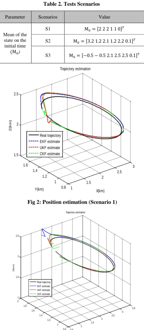
Table 2. Tests Scenarios

Parameter Scenarios Value

Mean of the state on the initial time

)

S1

S2

S3

Fig 2: Position estimation (Scenario 1)

Fig 3: Position estimation (Scenario 2)

Fig 4: Position estimation (Scenario 3)

The real trajectory of Target and estimation of position with EKF, UKF and CKF algorithms have shown in three dimensions at figures of 1, 2, and 3.

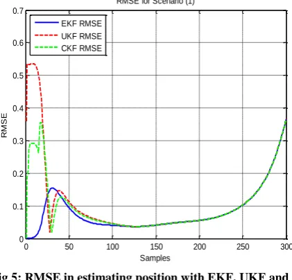
The performance of filters with using of root mean square error (RMSE) for each running simulation which is given by:

(21)

Where is Monte Carlo runs number,

is estimation for j Monte Carlo runs on (t) time and is true value.

In table 3 have listed the root mean square errors. RMSE (mean of position errors) of three tested methods in good initialize for EKF, UKF and CKF (Scenario 1) and in bad initialize (Scenario 2) and (Scenario 3) over 500 Monte Carlo runs.

Table 3. RMSEs of estimating the position in kilometers

Algorithm RMSE

scenario 1

RMSE scenario 2

RMSE scenario 3

EKF 0.1066 0.1912 0.7993

UKF 0.1687 0.1076 0.5644

CKF 0.1310 0.1075 0.3689

1 1.5

2 2.5

3

0.8 1 1.2 1.4 1.6 1.5

2 2.5

X(km) Trajectory estimation

Y(km)

Z

(k

m

)

Real trajectory EKF estimate UKF estimate CKF estimate

0.5 1

1.5 2

2.5 3

3.5

0.8 1 1.2 1.4 1.6 1.8 2 1 1.5 2 2.5

X(km) Trajectory estimation

Y(km)

Z

(k

m

)

Real trajectory EKF estimate UKF estimate CKF estimate

0 0.5

1 1.5

2 2.5

3

-0.5 0 0.5 1 1.5

0 0.5 1 1.5 2 2.5 3 3.5

X(km) Trajectory estimation

Y(km)

Z

(k

m

)

Fig 5: RMSE in estimating position with EKF, UKF and CKF (Scenario 1)

Fig 6: RMSE in estimating position with EKF, UKF and CKF (Scenario 2)

Fig 7: RMSE in estimating position with EKF, UKF and CKF (Scenario 3)

5.

CONCLUTION

In this paper, state estimation introduced for target tracking problems in three dimensions. Firstly State and measurement equations were obtained for target tracking problems. Then, the measurements (LOS angles in azimuth and elevation between pursuer and evader) that contaminated by high degree of noise are estimated using Extended Kalman filter (EKF), Unscented Kalman filter (UKF) and Cubature Kalman Filter (CKF) techniques. The filtering algorithms created in MATLAB have been tested under various scenarios. The results obtained which the efficiency of EKF has better performance due to least RMSE to compare with the UKF and CKF. But, the performance EKF algorithm has been dramatically decreased when initialization (initial state assumption) is not good, which in this condition CKF method provides a more accurate approximation.

6.

REFERENCES

[1] Goutam Chalasani,, Shovan Bhaumik 2011 “Bearing Only Tracking Using Gauss-Hermite Filter” 978-1-4577-2119- IEEE

[2] S.Sadhu, S.Bhaumik, and T.K.Ghoshal, Dec 18-21, 2004 “Evolving homing guidance configuration with Cramer Rao bound,” Proceedings 4th IEEE International Symposium on Signal Processing and Information Technology, Rome,

[3] T.L. Song, and J.L. Speyer, 1985 “A stochastic analysis of a modified gainextended Kalman filter with applications to estimation with bearings only measurements,” IEEE Transactions on Automatic Control, vol 30, no. 10, pp. 940-

[4] S. Koteswara Rao, K.S. Linga Murthy, and K. Raja Rajeswari, 2010. “Data fusion for underwater target tracking”, IET Radar Sonar Navigation, vol. 4, no. 4, pp. 576-585

[5] K. Dogancay, 2005 “Bearings-only target localization using total least squares,” Signal Process, vol. 85, pp. 1695-1710.

[6] R. E. Kalman, 1960 “A new approach to linear filtering and prediction problems,” ASME J. Basic Eng.,

[7] Jouni Hartikainen, Arno Solin, and Simo Särkkä, August 2011 “Optimal filtering with Kalman filters and smoothers” Aalto-Finland,.

[8] R. Karlsson and F. Gustafsson, , 2001 “Range estimation using angle-only target tracking with particle filters”, Proc. American Control Conference, pp.3743 – 3748. [9] B. L. Scala, M. Morelande, , 2008 “An Analysis of the

Single Sensor Bearings-Only Tracking Problem” Radar- Con

[10]Mallick, M., Morelande, M.R., Mihaylova, L, Arulampalam, S., Yan, 2012 “Comparison of Angle-only Filtering Algorithms in 3D using Cartesian and Modified Spherical Coordinates” 15th International Conference on. IEEE, p. 1392-1399.

[11]Aidala, V. J. Jan. 1979, Kalman filter behavior in bearings-only tracking applications. IEEE Transactions on Aerospace and Electronic Systems, AES-15, 29—39. [12]Nardone, S. C., Lindgren, A. G., and Gong, K. F. Sept.

1984 Fundamental properties and performance of

0 50 100 150 200 250 300

0 0.1 0.2 0.3 0.4 0.5 0.6 0.7

RMSE for Scenario (1)

Samples

R

M

S

E

EKF RMSE UKF RMSE CKF RMSE

0 50 100 150 200 250 300

0 0.1 0.2 0.3 0.4 0.5 0.6 0.7

RMSE for Scenario (2)

Samples

R

M

S

E

EKF RMSE UKF RMSE CKF RMSE

0 50 100 150 200 250 300

0 0.5 1 1.5 2 2.5 3 3.5 4 4.5

RMSE for Scenario (3)

Samples

R

M

S

E

Transactions on Automatic Control, AC-29, 9, 775— 787.

[13]Wan, E. A. and van der Merwe, R. 2001 “The unscented Kalman filter. In S. Haykin (Ed.), Kalman Filtering and Neural Networks” Hoboken, NJ: Wiley, ch. 7, pp. 221— 280.

[14]K.Radhakrishnan, A. Unnikrishnan, K.G Balakrishnan, 2010 “Bearing only Tracking of Maneuvering Targets using a Single Coordinated Turn Model” International Journal of Computer Applications.

[15]Julier, S.J., and Uhlmann, J.K, 1997 “A New Extension of the Kalman Filter to Nonlinear Systems,” Proceedings of AeroSense: The 11th Int. Symposium. On Aerospace/Defense Sensing, Simulation and Controls [16]Bar-Shalom, Y., Li, X.-R., and Kirubarajan, T, 2001.

Estimation with Applications to Tracking and Navigation. Wiley Interscience.

[17]S. J. Julier and J. K. Uhlmann,2004 “Unscented filtering and nonlinear estimation,” Proceedings of the IEEE, vol. 92, no. 3, pp. 401–422, 200

[18]Julier, S.J., and Uhlmann, J.K, 1997, A New Extension of the Kalman Filter to Nonlinear Systems, Proceedings of AeroSense: The 11th Int. Symposium. On Aerospace/Defense Sensing, Simulation and Controls. [19]Daum, F., 2005, Nonlinear Filters: Beyond the Kalman

Filter, IEEE A&E Systems Magazine, Vol. 20., No. 8. [20]Arasaratnam, I. and Haykin, S. June 2009, Cubature

Kalman filters. IEEE Transactions on Automatic Control, 54, 6 , 1254—1269.

[21]Arasaratnam, I. and Haykin, S. Oct 2009. Cubature Kalman filtering: A powerful tool for aerospace applications. Presented at the International Radar Conference, Bordeaux, France.Wu, Y., et al.

[22]Aug. 2006A numerical-integration perspective on Gaussian filters. IEEE Transactions on Signal Processing, 54, 8 , 2910—2921