Munich Personal RePEc Archive
Loss Given Default Modelling under the
Asymptotic Single Risk Factor
Assumption
Kim, Joocheol and Kim, KiHyung
Yonsei University
17 November 2006
Loss Given Default Modelling under the
Asymptotic Single Risk Factor Assumption
Joocheol Kim
∗
,
Department of Economics, Yonsei University, 134 Shinchon-dong, Seodaemun-ku, Seoul, 120-749, Korea
KiHyung Kim
School of Business, Yonsei University, 134 Shinchon-dong, Seodaemun-ku, Seoul, 120-749, Korea
Abstract
The proposals of the Basel Committee on Banking Supervision for the revision of minimum requirements for bank’s risk capital leave the quantification of loss-given-default (LGD) parameter used for capital calculation unspecified. This paper proposes a new methodology for incorporating LGD parameter explicitly into the Basel risk weight function. Numerical examples based on the new methodology are compared to the current proposals of the Basel committee on Banking Supervision.
∗ Corresponding author.
1 Introduction
The proposals of the Basel Committee on Banking Supervision (the Com-mittee hereafter) for the revision of minimum requirements for banks’ risk capital have raised a lot of discussions how to quantify the loss given default (LGD) used for capital calculations. In particular, a number of interested par-ties including industry associations and national supervisors have asked the Committee to further elaborate on the so-called “downturn LGD” standard described in the proposals, which requires that estimated downturn LGD must “reflect economic downturn conditions where necessary to capture the relevant risks.” In September 2004, the Committee’s Capital Task Force and its Ac-cord Implementation Group agreed to set up the LGD working group to share views and consider appropriate approaches to meeting the requirements re-garding LGD estimates. After several months, the LGD working group have drawn the following three findings.
First, the potential for realized recovery rates (which is one minus the LGD) to be lower than average during times of high default rates may be a material source of unexpected credit losses for some exposures or portfolios. Failing to account for this possibility risks understating the capital required to cover un-expected losses. Second, data limitations pose an important challenge to the estimation of LGD parameters in general, and of LGD parameters consistent with economic downturn conditions in particular. Third, there is currently lit-tle consensus within the banking industry with respect to appropriate methods for incorporating downturn conditions in LGD estimates. (See Basel Commit-tee on Banking Supervision(2005))
While a significant body of academic and practitioner research suggests that systematic volatility in recovery rates is a potentially important source of unexpected credit losses for some exposures or portfolios, only a couple of research papers propose a way to incorporate the effects of systematic risk on recovery rates directly into estimated LGD (for instance, Pykhtin(2003), Dirk(2004)).
mapping function. Finally numerical examples based on a specific assumption on the the distributional form are compared to the original Basel Committee’s framework.
2 A Brief Review of IRB Approach
There are always some borrowers that fail to meet their obligations. The losses caused by default events fluctuate every year, depending on the number and severity of default events. Financial institutions never know in advance the losses that they will experience in a particular year. They can, however, fore-cast the expected loss by estimating the proportion of obligors that might default within a given time horizon, multiplied by the outstanding exposure at default and once more multiplied by the percentage of exposure that will not be recovered by sale of collateral. The expected loss can then be written as
IE[L] =P D·EAD· LGD (1) where P D is the probability of default, EAD is the exposure at default, and LGDis the loss (rate) given default. These three random variables are the risk parameters upon which the internal ratings based (IRB) approach is built.
Under the asymptotic single risk factor (ASRF) model assumed by the IRB approach (Gordy(2003)), the loss rate for a well diversified portfolio depends only on the (single) systematic risk factor and not on idiosyncratic risk factors associated with individual exposures. If X denotes the systematic risk factor and L denotes the loss rate on the exposure, financial institutions must hold, for each exposure,IE[L|X =α] percentage of provisions and capital to satisfy 99.9% VaR(Value-at-Risk) target, whereαis 99.9th percentile of the standard normal distribution.
By introducing an indicator variable D (which is 1 if default, 0 otherwise), IE[L|X =α] can be written as
IE[L|X =α] =P(D= 1|X =α)·IE[L|D= 1, X =α] (2)
The first term is the conditional default probability (CPD) of the exposure given the 99.9th percentile adverse movement of systematic risk factor and the second term is the conditional loss given default based on the same adverse movement of X. The conditional loss given default(CLGD) can be thought as the so-called “downturn LGD”.
In the IRB approach, financial institutions are not required to estimate CPDs directly. Instead, a mapping function is provided by the Basel Committee to calculate an exposure’s conditional default probability from their own estimate of expected default probability.
CP D = Φ
Ã
Φ−1(P D) +√ρ·Φ−1(0.999)
√
1−ρ
!
where Φ(x) is a standard normal cumulative density function, Φ−1(p) is the inverse of this function, and ρ is an asset-value-correlation (AVC) parameter prescribed by the Basel Committee.
Combining equations (2) and (3) produces the following expression for the conditional loss (rate) of an exposure.
IE[L|X =α] = Φ
Ã
Φ−1(P D) +√ρ·Φ−1(0.999)
√
1−ρ
!
·CLGD (4)
This formula forms the core of the IRB risk-weight functions that appear in the Framework Document.
In summary, the IRB approach allows financial institutions to use their own internal estimates for key drivers (such as the borrower’ probability of de-fault, exposure at dede-fault, and loss given default) to calculate the required risk capital, subject to meeting certain conditions and the supervisory ap-proval. These risk parameters are converted into risk weights and regulatory capital requirements by means of risk weight formulas specified by the Basel Committee1.
1 This section is largely based on “Background note on LGD quantification” from
3 LGD modelling
In finance, it is frequently assumed that the asset return is distributed as a normal random variableS ∼N(µ, σ2), whereµand σ are mean and standard
deviation, respectively. Under the Internal Ratings Based (IRB) approach, the asset return is considered as a latent variable and the asymptotic single risk factor model (Gordy(2003))
S =µ−b X +ω ξ (5)
is assumed where X ∼ N(0,1) and ξ ∼ N(0,1). The random variable X denotes the systematic risk factor which is common to each obligor and the random variable ξ represents the idiosyncratic risk factor associated with in-dividual obligor2. Idiosyncratic shock ξ is assumed to be independent from
the systematic risk factor X.
Alternatively, the asset return is standardized and is given by
Y = S−µ σ =−
√ρ X+q
1−ρ ξ (6)
where √ρ=b/σ denotes the exposure to the common systematic risk factor. The standardized return Y can be interpreted as the obligor’s ability to pay debts.
In the IRB approach, default events are assumed to occur if Y ≤C, where C is a certain critical value. In other words, when the standardized return Y, or the ability-to-pay variable, of an obligor is less than or equal to some critical value, the obligor is classified as default. The probability of default can then be expressed as
P(Y ≤C) =P(−√ρ X+q1−ρ ξ ≤C) (7)
For practical purposes, the probability of default needs not to be calculated theoretically. Rather, it is usually estimated from historical experiences of default.
The conditional probability of default given that the systematic risk factor X is set to some known valueα is represented as
P(Y ≤C|X =α) =P
Ã
ξ≤ C+
√ρ α √
1−ρ
!
(8)
which is equivalent to (3), assuming that the critical valueC is Φ−1(P D) and α is the 99.9th percentile from the standard normal distribution.
While the ability-to-pay variableY only plays a role that determines whether an obligor defaults or not in the IRB framework, Y may also be interpreted as information variable containing the capability of an obligor to pay debts given default. If a certain defaulted obligor’s ability-to-pay variableY is much less than the other defaulted obligor’sY, then the former might be considered to have much less ability to pay debts than the latter does. Thus, we may postulate that the smaller the ability-to-pay variable Y is, the larger the loss occurs when an obligor defaults. In that case, we may express the loss rate due to an obligor as a monotonically decreasing function of Y.
L=f(Y) (9)
Now the expected loss in (2) can be restated as
IE[L|X =α] =IE[f(Y)|Y ≤C, X =α]·P(Y ≤C|X =α) (10)
which states that the bank’s regulatory capital can be calculated as a product of the conditional expectation of loss given default and the conditional prob-ability of default. With the help of the LGD modelling in this section, the conditional expectation of loss given default can be written as
IE[f(−√ρ X+q1−ρ ξ)| −√ρ X+q1−ρ ξ≤C, X =α] (11)
In order to find the explicit expression for the conditional expectation of loss given default when the systematic risk factor X is set to α, the joint prob-ability of loss, default and systematic risk factor, P(L = t, D = 1, X = α), should be specified. Though this joint probability seems to contain three ran-dom variables at a first glance, the modelling of this section makes this joint probability having only two random variables, X and ξ. Thus the joint prob-ability can be obtained by transforming of joint pdf of X and ξ, and can be restated as
P(−√ρ X+q1−ρ ξ =f−1(t),−√ρ X+q1−ρ ξ ≤C, X =α) (12)
And the conditional pdf ofP(L=t|D= 1, X =α) can be explicitly found by
P(Y =f−1(t)|Y ≤C, X =α) = φ(
f−1(t)+√ρα
√
1−ρ )
Φ(C√+√ρα
1−ρ )
· √ 1
1−ρ, −∞< f
−1(t)≤C
(13) where Y =−√ρ X+√1−ρ ξ and C= Φ−1(P D). The detailed derivation of (13) is in the Appendix.
factor X is set toα can be calculated by
IE[f(Y)|Y ≤C, X =α] =
Z C
−∞
f(u) φ(
u+√ρα
√
1−ρ )
Φ(C√+√ρα
1−ρ )
· √ 1
1−ρdu (14)
4 Numerical example
In the previous section, we suggest that the loss rate can be modelled as a monotonically decreasing function of an obligor’s ability-to-pay variable Y.
L=f(Y) (15)
The choice off depends on the characteristics of loss (rate) given default. In practice, the usual choice of the loss given default distribution is a Beta dis-tribution with two parametersa andb. This choice can be justified by the fact the support of the distribution is [0,1], which is appropriate for modelling the (loss) rate. Also, the Beta distribution represents various shapes through the parameters a and b. Finally, it is straightforward to estimate the parameters a and b by moment matching given the historical average and variance of the realized loss data.
In this section, we compare the risk capital charges by the current Basel II formula with those by specific assumption of the functional formf. Specifically we assume the following
L=f(Y) =IB−1(Φ(C)−Φ(Y)
Φ(C) ), Y < C (16)
where IB−1 denotes inverse of the beta cumulative distribution function. The modelling of this paper is still valid for other choices of f 3.
The exposure to the common systematic risk factor ρ involved in the risk weight function were set according to the rule for corporate exposures (See Basel Committee on Banking Supervision(2003)), i.e.
ρ=ρ(P D) = 1−e−
50P D
1−e−50 0.12 +
Ã
1−1−e−
50P D
1−e−50
!
0.24 (17)
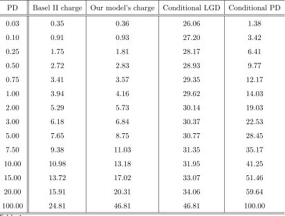
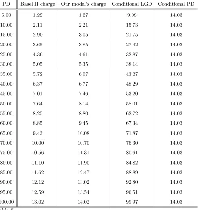
Table 1 lists the results in the case of varying PDs with fixed expected LGD. In Table 1, our model’s charge is calculated by IE[L|X =α]−EL. Table 2, which list the results in the case of fixed PD with varying expected LGDs also have the same implication as Table 1. The implication from both Table 1 and Table 2 supports the finding of LGD working group in the Basel Committee that the potential for realized LGDS to be lower than average during times of high default rates may be a material source of unexpected credit losses for
3 In case that there exists no inverse function of f, generalized inverse function of
some exposures or portfolios. Since the capital charges calculated by a new methodology suggested in the paper are always greater than the original Basel charges, the suggested methodology may serve as a remedy for the original Basel risk weight function.
Just by changing the conditional LGD with the suggested LGD formula, we confirm the relationship
IE[L|X =α] =CLGD·Φ
Ã
Φ−1(P D) +√ρ·Φ−1(0.999)
√
1−ρ
!
(18)
PD Basel II charge Our model’s charge Conditional LGD Conditional PD
0.03 0.35 0.36 26.06 1.38
0.10 0.91 0.93 27.20 3.42
0.25 1.75 1.81 28.17 6.41
0.50 2.72 2.83 28.93 9.77
0.75 3.41 3.57 29.35 12.17
1.00 3.94 4.16 29.62 14.03
2.00 5.29 5.73 30.14 19.03
3.00 6.18 6.84 30.37 22.53
5.00 7.65 8.75 30.77 28.45
7.50 9.38 11.03 31.35 35.17
10.00 10.98 13.18 31.95 41.25
15.00 13.72 17.02 33.07 51.46
20.00 15.91 20.31 34.06 59.64
[image:12.595.95.507.75.388.2]100.00 24.81 46.81 46.81 100.00
Table 1
PD Basel II charge Our model’s charge Conditional LGD Conditional PD
5.00 1.22 1.27 9.08 14.03
10.00 2.11 2.21 15.73 14.03
15.00 2.90 3.05 21.75 14.03
20.00 3.65 3.85 27.42 14.03
25.00 4.36 4.61 32.87 14.03
30.00 5.05 5.35 38.14 14.03
35.00 5.72 6.07 43.27 14.03
40.00 6.37 6.77 48.29 14.03
45.00 7.01 7.46 53.20 14.03
50.00 7.64 8.14 58.01 14.03
55.00 8.25 8.80 62.72 14.03
60.00 8.85 9.45 67.34 14.03
65.00 9.43 10.08 71.87 14.03
70.00 10.00 10.70 76.30 14.03
75.00 10.56 11.31 80.61 14.03
80.00 11.10 11.90 84.82 14.03
85.00 11.62 12.47 88.89 14.03
90.00 12.12 13.02 92.80 14.03
95.00 12.59 13.54 96.51 14.03
[image:13.595.100.508.78.512.2]100.00 13.02 14.02 99.97 14.03
Table 2
0 0.2
0.4 0.6
0.8 1
0 0.5
1 −0.2 0 0.2 0.4 0.6
LGD PD
[image:14.595.141.425.283.491.2]Capital Charge
5 Concluding Remarks
The proposals of the Basel Committee on Banking Supervision for the revision of minimum requirements for bank’s risk capital leave the quantification of loss-given-default (LGD) parameter used for capital calculation unspecified.
We propose a so-called mapping function from the long-term average LGD to downturn LGD, similar to the Basel Committee’s mapping function from the long-term probability of default to the conditional default probability. In particular, the proposed mapping function is quite general so that large number of specific assumptions on the functional form can be applied to the mapping function. Finally numerical examples based on a specific assumption on the the functional form are compared to the original Basel Committee’s framework.
A Appendix
Let
Y1=−√ρ X (A.1)
Y2=−√ρ X+
q
1−ρ ξ (A.2)
X=−√Y1
ρ (A.3)
ξ=Y√2−Y1
1−ρ (A.4)
The Jacobian of the transformation is
|J|=
¯ ¯ ¯ ¯ ¯ ¯ ¯ − 1
√ρ 0
−√1
1−ρ
1
√
1−ρ
¯ ¯ ¯ ¯ ¯ ¯ ¯
= √ 1
ρ√1−ρ (A.5)
The joint pdf of (Y1, Y2) is
fY1,Y2(y1, y2) = φ(−
y1
√ρ)φ(√y2−y1 1−ρ)
Ã
1
√ρ√
1−ρ
!
(A.6)
which is N(ρy2, ρ(1−ρ))·N(0,1).
The marginal pdf ofY1 is
fY1(y1) =
Z ∞
−∞
fY1,Y2(y1, y2)dy2 =φ(−
y1
√ρ)√1
ρ (A.7)
which is N(0, ρ).
The marginal pdf ofY2 is
fY2(y2) =
Z ∞
−∞
fY1,Y2(y1, y2)dy1 =φ(y2) (A.8)
which is N(0,1).
The conditional probability ofY2 givenY1 is
P(Y2 =y2|Y1 =y1) = φ(
y2−y1
√
1−ρ)
Ã
1
√
1−ρ
!
which is N(y1,1−ρ).
The conditional probability ofY1 givenY2 is
P(Y1 =y1|Y2 =y2) = φ(
y1 −ρy2
√ρ√
1−ρ)
Ã
1
√ρ√
1−ρ
!
(A.10)
which is N(ρy2, ρ(1−ρ)).
Using this transformation, we can describeP(L=t|Y < C, X =α) as follow-ing
P(L=t|Y < C, X =α) = P(L=t, Y < C, X =α) P(Y < C, X =α)
= P(L=t, Y < C, X =α) P(Y < C|X =α)P(X =α)
= P(Y2 < C, Y1 =−
√ρα)
P(Y2 < C|Y1 =−√ρα)P(Y1 =−√ρα) − ∞
< f−1(t)≤C
(A.11)
LetY2 =f−1(t), andP(Y2 < C|Y1 =−√ρα) denotes the CPD. We can derive
(13) by substituting (A.6) and (A.8) in this equation,
P(Y =f−1(t)|Y ≤C, X =α) = φ(
f−1(t)+√ρα
√
1−ρ )
Φ(C√+√ρα
1−ρ )
· √ 1
1−ρ, −∞< f
−1(t)≤C
References
[1] Basel Committee on Banking Supervision. (2003). The New Basel Capital Accord. Bank for International Settlements, July 2003.
[2] Basel Committee on Banking Supervision. (2004). Modifications to the capital treatment for expected and unexpected credit losses. Bank for International Settlements, January 2004
[3] Basel Committee on Banking Supervision. (2005). Guidance on Paragraph 468 of the Framework Document. Bank for International Settlements, July 2005.
[4] Gordy, M. B. (2000). A comparative anatomy of credit risk models, Journal of Banking and Finance, Vol 24, pp.119-149.
[5] Gordy, M. B. (2003). A risk-factor model foundation for ratings-based bank capital rule. Journal of Financial Intermediation, Vol 12, pp. 199-232.
[6] Pykhtin, M. (2003). Unexpected recovery risk. Risk, Vol 16, No 8. pp. 74-78.