Design an Optimal PID Controller using Artificial Bee Colony and Genetic Algorithm for Autonomous Mobile Robot

Design an Optimal PID Controller using Artificial

Bee Colony and Genetic Algorithm for Autonomous

Mobile Robot

Ramzy S. Ali

Ammar A. Aldair

Ali K. Almousawi

Engineering College

University of Kufa, Iraq

ABSTRACT

Target tracking is a serious function for an autonomous mobile robot navigating in unknown environments such as disaster areas, projects sites, and any dangerous place which the human cannot reach. This paper deals with modified the parameters of PID controller using Artificial Bee Colony (ABC) and Genetic Algorithm (GA) for path tracking of autonomous mobile robot. Two PID control are designed, one for speed control and the other for azimuth control. The MATLAB program is used to simulate the autonomous mobile robot model with optimal PID controllers, ABC algorithm and GA. To test the effectiveness of the proposed controllers, two path trajectories have been chosen: circular path and sine wave path. The results have clearly shown the effectiveness and good performances of the PID controllers which are tuned using ABC algorithm than using GA.

General Terms

Control system design for autonomous robot system.

Keywords

Autonomous mobile robot, artificial bee colony, genetic algorithm, PID controllers.

1.

INTRODUCTION

Mobile robot manipulators are mobile robot bases with at least one mounted robot arm which function in an integrated manner. The purpose of the mobile manipulator is to reach concrete locations in its environment and to pick up objects. There are two applications of using a mobile robot manipulator (MRM). The first one: using the MRM in unstructured environments, especially in the scenario that is unsuitable for human beings. The second application: using the MRM to transport objectives and tools in an already known industrial environment. Autonomous mobile robots are able to carry out many functions in dangerous sites where humans cannot reach, such as sites where harmful gases or high temperature are present, a hard environment for humans. Home assistant robots are expected to support daily activities at home. In all these examples robots have to move to their destination in order to perform their functions. For this purpose they need to be able to recognize the changes of environment using various sensors and cameras, and be equipped with a motion planning method in order to avoid collision with obstacles or other robots. In this work, the target tracking control issue are studied to improve the performances of the mobile robot.

The PID controllers are widely being used in the industries for process control applications. Even for complex industrial control system, the industries use the PID control module to build the main controller. The merit of using PID controllers

lie in its simplicity of design and good performance including low percentage overshoot and small settling time for normal industrial processes [1]. Several formulas have been suggested to select the suitable parameters of PID controller. Zielger-Nichols tuning method was introduced in 1942 to tune the PID control parameters. This tuning method can be applied when the plant model is given by a first-order plus dead time. Many variants of the traditional Ziegler-Nichols PID tuning methods have been proposed such as the Chien-Hrones-Reswick formula, Cohen-Coon formula, refine Ziegler-Nichols tuning formula, Wang-Juang-Chan formula and Zhuang-Atherton optimum PID controller [2]. The main problem of use the PID controller is the correct choice of the suitable control parameters to improve the transient response of the controlled system. Using other words, the random setting for the parameters of PID controller, the controller may not provide the required control performance, when there are variations in the plant parameters and operating conditions.

Many authors proposed different algorithm to tune the parameters of PID controller. The genetic algorithm was used to modify the PID controller [3-5]. The particle swarm optimization method was used to tune the parameters of PID controller [6-8]. Some authors used Artificial Bees Colony (ABC) optimization algorithm for regulation parameters of PID controller [9].

In this paper, two algorithms (ABC and GA) are used to tune the parameters of PID controller to force the Autonomous mobile robot to follow the specific trajectory. Two PID control are designed, one for speed control and the other for azimuth control. The control signal is applied to mobile robot system for obtaining smooth path tracking of two wheeled differential which drive the mobile robot. The MATLAB program is used to simulate the autonomous mobile robot model with optimal PID controllers; ABC algorithm and GA.

2.

AUTONOMOUS MOBILE ROBOT

MODEL

Modeling of a differential drive mobile robot platform consists of kinematic and dynamic modeling. Each part of this system’s modeling will be explained separately. After getting an accurate model, a complete system is simulated using an MATLAB program package.

2.1

Kinematic Model of Mobile Robot

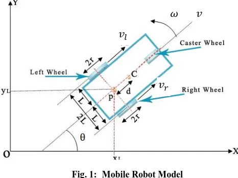
Kinematics refers to the evolution of the position, and velocity of a mechanical system, without referring to its mass and inertia. The kinematic scheme of the mobile robot consists of a platform driven by two driving wheels mounted on same axis with independent actuators and one free wheel that is called a castor. The movement of mobile robot is done by changing the relative angular velocities of driving wheels. The assumptions are that the whole body of robot is rigid and motion occurs without sliding. Its wheel rotation is limited to one axis. Therefore, the navigation is controlled by changing speed on either side of the robot. The kinematics scheme of the differential drive mobile robot is as shown in Figure 1 where {O , X , Y } are the global coordinate and {P, , } are the local coordinate which are fixed to the robot with its centre P between the two wheels, r is the radius of each wheel and 2L is the distance between two driving wheels, ω is the angular velocity of the mobile robot, and are thevelocity of the left and right driving wheel, the angle θ indicates the orientation of the robot, C represented the centre of the mobile robot, d is the distance from center of mobile robot to origin P.

According to the motion principle of rigid body kinematics, the motion of a two wheel differential drive mobile robot can be described using Eq. (1) and Eq. (2), where and are angular velocities of the left and right driving wheels respectively [10].

The nonholonomic constraint equation of the robot is as following:

Substitution equation (1) in (2) yield :

Additionally, we can define the dynamic function of the robot as follows.

Re-arranged equation (5) as a matrix yield:

where and : denote the velocity of the robot in the direction of X-axis and Y-axis, respectively.

2.2

Dynamic Model of mobile robot

The design procedure will depend on the Lagrange-Euler differential equation of dynamics which is shown below [10]:

τ

)

(

K

)

(

G

)

(

F

w

)

,

(

w

)

(

M

q





C

q

q





q





q



q

(7)

F is a 2×1 vector which holds the friction force and G is a 2×1 vector which holds the gravitation force acting upon the robot, but because of the assumptions that the robot does not slip and it moves on flat ground, both forces are set to zero.

With the assumptions that the robot does not slip, not disturbance, and it moves on flat ground; the third, fourth and fifth bound are set to zero. Then the equation (3.9) becomes

:

τ

)

(

K

w

)

,

(

w

)

(

M

q





C

q

q





q

(8)

where W = [ ]T , input torques on the wheels τ = [τr, τl]T , M is a 2×2 symmetric and positive definite inertia matrix, which describe as

M

=

where

C is a 2×2 matrix which holds the centripetal forces which affect upon the wheels, where c equals the viscous friction of the wheels against the ground. K is a 2×2 input transformation matrix for the torque vector, where k is the gain constant for

each torque input (

K



k

I

Fig. 1:

To convert Eq. (8) to the canonical state-space dynamics model with respect to the state vector w, the equation becomes:

₍₉₎

3.

STRUCTURE OF PID CONTROLLER

The PID term refers to the first letter of the names of the individual terms that make up the standard three term controller. These are: P for the proportional term; I for the integral term and D for the derivative term in the controller. Appropriate tuning of these parameters will improve the performance of the plant, reduce the overshoot, eliminate steady state error and increase stability of the system.

The main problem of that simple controller is the correct choice of the PID gains. By using fixed gains, the controller may not provide the required control performance, when there are variations in the plant parameters and operating conditions. Therefore, the tuning process must be performed to insure that the controller can deal with the variations in the plant.

Because most PID controllers are adjusted on-site, many different types of tuning rules have been proposed in the literature. Using these tuning rules, delicate and fine tuning of PID controllers can be made on-site. Also, automatic tuning methods have been developed and some of the PID controllers may possess on-line automatic tuning capabilities.

In this work, two PID controllers are proposed for motion control of autonomous mobile robot. The first one of PID controller is used to control the velocity and another for controlling azimuth of the mobile robot. The velocity and azimuth of the robot are controlled by manipulating the torques for the left and the right-wheels which illustrate on the same Figure 2.

The x desired , y desired and desired are considered as the input signal to proposed system. Error of

arecalculated from equation 10:

(10)

where ; : are the actual x, y and the actual azimuth of the robot, respectively. Then convert the Cartesian Coordinate into Polar Coordinate to calculate the distance error as shown below:

(11

)

The distance error and the azimuth error are considered as the inputs for PID controller, and the driving torques required for controlling the two wheels ( and ) are considered as outputs.

In this work two intelligent algorithms are studied to find the optimal parameters of the PID controllers: first algorithm is GA and the second algorithm is ABC. Each algorithm is described in detail in the following subsection.

4.

THE GENETIC ALGORITHM

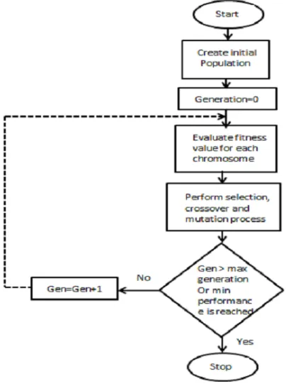
The Evolutionary Algorithm (EA) is an optimization algorithm is used to search for optimal solutions to a problem. This algorithm operates on a population of potential solutions applying the principle of survival of the fittest to produce better and better approximations to a solution. Evolutionary algorithms provide a universal optimization technique that mimics the type of genetic adaptation that occurs in natural evolution. Unlike specialized methods designed for particular types of optimization tasks, they require no particular knowledge about the problem structure other than the objective function itself. At each iteration step, a new set of approximations is assumed by the process of selecting individuals according to their level of fitness in the problem domain and breeding them together using operators, such as mutation, crossover and selection, borrowed from natural genetics in order to generate the new generations [11]. The GA flowchart is shown in Figure 3.

In the case of using a GA method to tune the PID gains to design the control system for the mobile robot, the fitness function used to evaluate the individuals of each generation can be chosen to be Mean Square Error (MSE)

where =No. of samples , k: sample time.

During the search process, the GA looks for the optimal setting of the PID controller gains which minimizes the fitness function (MSE).

This function is considered as the evolution criteria for the GA. The choice of this fitness function has the advantage of avoiding cancellation of positive and negative errors.

Desired Path

𝑑, 𝑑, 𝑑

Error Calculation

Cartesian to polar

𝑑 _{First PID Controller}

Second PID Controller

Mobile Robot System 𝑢

𝑢𝑙

Actual path

𝑎 𝑢𝑎𝑙, 𝑎 𝑢𝑎𝑙, 𝑎 𝑢𝑎𝑙

Each chromosome represents a solution of the problem and hence it consists of three genes: the first one is the Kp value, the second on is Ki value and last one is the Kd value: Chromosome vector = [Kp Ki Kd]. It must be noted here that the range of each gain must be specified. Figure 4 show the learning phase of the PID controllers which connected with autonomous mobile robot.

5.

ARTIFICIAL BEE COLONY

ALGORITHM

The Artificial Bee Colony (ABC) algorithm was recently proposed by Karaboga [12]. It proposed to simulate the foraging behavior of honey bee colonies. In this Algorithm, the foraging bees are divided into three categories: Employed bees (which go to the food source), Onlookers bees (which wait on the dancing area to making decision to choose a food source depend on the collecting information by employed

bees) and Scout bees (which carry out random search for new food source near the hive. Employed bees share information about food sources by dancing in the designated dance area inside the hive. The nature of dance is proportional to the nectar content of food source just exploited by the dancing bee. Onlooker bees watch the dance and choose a food source according to the probability proportional to the quality of that food source. Therefore, good food sources attract more onlooker bees compared to bad ones. Whenever a food source is exploited fully, all the employed bees associated with it abandon the food source and become scout. Scout bees can be visualized as performing the job of exploration, where as employed and onlooker bees can be visualized as performing the job of exploitation.

ABC algorithm, as an iterative algorithm, starts by associating each employed bee with randomly generated food source (solution). In each iteration, each employed bee discovers a food source in its neighborhood and evaluates its nectar amount (fitness) using Equation (13), and computes the nectar amount of this new food source:

where is the jth food source, is the jth randomly

selected food source, j is a randomly chosen parameter index and is a random number within the range [-1, 1]. The

range of this parameter can make an appropriate adjustment on specific issues.

Onlooker bees observe the waggle dance in the dance area and calculate the profitability of food sources, then randomly select a higher food source. After that onlooker bees carry out randomly search in the neighbourhood of food source. The flowchart for ABC algorithm is given in Figure 5.

The quantity of a food source is evaluated by its profitability and the profitability of all food sources. is determined by the formula:

where is the fitness value of . This value is proportional to the nectar amount of the food source in the position i and is the number of food source which is equal to the number of employed bees.

Fig. 3: Genetic Algorithm architecture

Desired Path

,

,

Error

Calculation

Cartesian to

polar

𝑑

_{First PID Controller}

Second PID Controller

Mobile Robot

System

𝑢

𝑢

Actual path

𝑎 𝑢𝑎𝑙

,

,

Cost function

Calculation

Genetic Algorithm

(GA)

The employed bee becomes a scout bee when the food source which is exhausted by the employed and onlooker bees is assigned as abandoned. In that position, scout generates randomly a new solution by Eq. (13):

𝑎 𝑑

Assume that the abandoned source is , then the scout discovers a new food source to be replace with .

6.

SIMULATION AND RESULTS:

For the autonomous mobile robot system discussed in Section 2, the numerical values are used in this simulation are given in Table 1.

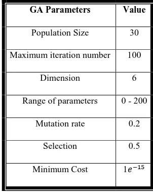
The simulation blocks that used for simulation trajectory tracking using GA-PID Controller is shown in Figure 5 (the same structure is used for simulation trajectory tracking using ABC-PID Controller). This Simulink is programmed as m file to achieve optimization with solving all the differential equations by using the order Runge-Kutta method and the control sampling period is 0.01s. The search space consists of six dimensions, three dimensions specified for first controller (velocity controller) and other three dimensions for the second controller (azimuth controller). The GA parameters values are shown in Table 2, while optimal tuned parameters of PID controllers are shown in Table 3.

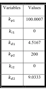
The ABC parameters values are shown in Table 4, while PID Controllers optimal tuned parameters using ABC algorithm are shown in Table 5.

Parameters Value Unit

1 m/s

r 0.05 m

L 0.1 m

d 0.1 m

1.8 Kg

0.1 Kg

m 2 Kg

0.0025 Kg.m2

0.001 Kg.m2

Value GA Parameters

30 Population Size

100 Maximum iteration number

6 Dimension

0 - 200 Range of parameters

0.2 Mutation rate

0.5 Selection

1 Minimum Cost

Fig. 5: The flowchart of ABC Algorithm

Table 1. numerical values of the mobile robot

In order to investigate the performance of two proposed controller, we compare the results of these controllers for tracking at two different paths to determine the better controller.

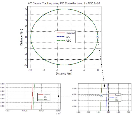
1) The circular trajectory given by a linear velocity

and desired azimuth given by

(15)

where and . Figure 6 shows the actual and desired path for circular path trajectory. Figures 7, 8 and 9 show the respectively.

Table 6 illustrates the MSE for circular trajectory tracking for two controllers.

Fig. 5: Simulation model for mobile robot trajectory tracking control using PID controllers

Variables

Values

99.4610

0.1287

4.5571

191.7988

1.3629

8.9214

Table 3 PID Controllers optimal tuned parameters using GA

Value ABC Parameters

40 Colony Size

100 Maximum iteration number

6 Dimension

5 Limit

5 scout production

Table 4. The ABC parameters values

Variables Values

100.0007

0

4.5167

200

0

9.0333

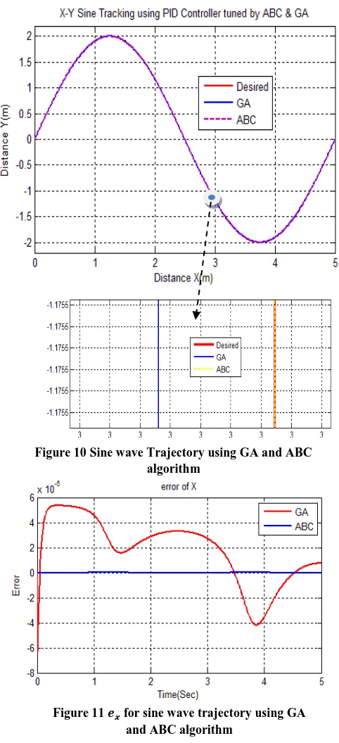
2) The sine wave trajectory given by a linear velocity

and desired x position , desired y position desired azimuth are given by

𝑎

Where

and .

Figure 10 shows the actual and desired path for sine wave path trajectory. Figures 11, 12 and 13 show the 𝑎 𝑑 respectively.

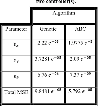
Table 7 illustrates the MSE for sine wave trajectory tracking for two controllers.

Fig. 9: for Circular Trajectory using GA and ABC algorithm

Algorithm

Parameter Genetic ABC

3.0332 1.6586

6.2711 2.6396

1.1911 5.7856

Total MSE 1.2911 1.6446

Table 6 MSE for circular trajectory tracking for two controllers.

Figure 12 for sine wave trajectory using GA Figure 10 Sine wave Trajectory using GA and ABC

algorithm

7.

CONCLUSION

Two optimization algorithms are used to find the optimal values of two PID controllers to solve the trajectory tracking of autonomous mobile robot. The obtained results show that the ABC algorithm is more effective than the genetic algorithm. For both tested trajectories path (circular trajectory and sine wave trajectory) the MSE when ABC used to tune the PID controllers parameters is less than the MSE when genetic algorithm used.

8.

REFERENCES

[1] Astrom, K.J. and T. Hagglund, PID controller: Therory, Design and Tuning 1995, USA: Instrument Society of America, Research Triangle Park.

[2] Xue, D., Y. Chen, and D.P. Atherton, Linear Feedback Control Analysis and Design with MATLAB. 2007, USA: The soceity for Industrial and Applied Mathematics

[3] Turki Y. Abdalla, S.J.A., Genetic Algorithm Based Optimal of a Controller for Trajectory Tracking of a Mobile Robot. Basrah Journal for Engineering Science, 2010. 1(1): p. 54-65.

[4] Ali, A.A., PID Parameters Optimization Using Genetic Algorithm TEchnique for Electrohydraulic Servo Control System. Intelligent Control and Automation, 2011. 2: p. 69-76.

[5] Gauri Mantri, N.R.K., Design and Optimization of Controller Using Genetic Algorithm. International Journal of Research in Engineering and Technology, 2013. 2(6): p. 926-930.

[6] Ali Tarique, H.A.G., Particle Swarm Optimization Based Turbine Control. Intelligent Control and Automation, 2013. 4: p. 126-137.

[7] Mahmud Iwan Solihin, L.F.T., Moey Leap Kean Tuning of PID Controller Using Particle Swarm Optimization in Proceeding of the International Conference on Advanced Science, Engineering and Information Technology. 2011: Bangi-Putrajaya, Malaysia.

[8] Gaing, Z.-L., A Particle Swarm Optimization Approach for Optimum Design PID Controller in AVR System. IEEE Transaction on Energy Conversion, 2004. 19(2): p. 384-391.

[9] El-Telbany, M.E., Tuning PID Controller for DC Motor: an Artifical Bees Optimization Approach International Journal of Computer Applications, 2013. 77(15): p. 18-21.

[10] Reched Dhaouadi, A.A.H., Dynamic Modelling of Differential-Drive Mobile Robots using Lagrange and Newton-Euler Methodologies: A Unified Framework. Advances in Robotics and Automation, 2013. 2(2): p. 1-7.

[11] S. Sumathi, T.H., Evolutionary Intelligence An Introduction to Theory and Applications with Matlab, ed. S.V. Berlin. 2007, German.

[12] D. Karaboga, B.B., A Powerful and Efficient Algorithm for Numerical Function Optinization: Artificial Bee Colony ABC Algorithm. . Journal Global Optimization, 2007. 39: p. 459-471.

Algorithm

Parameter Genetic ABC

2.22 1.9775

3.7281 2.09

6.76 7.37

Total MSE 9.8481 5.792

Fig. 13: for sine wave trajectory using GA and ABC algorithm