Testing Trade led Growth Hypothesis for Romania

Munich Personal RePEc Archive

Testing Trade-led-Growth Hypothesis for

Romania

Pop-Silaghi, Monica Ioana

Babes-Bolyai University

March 2006

Online at

https://mpra.ub.uni-muenchen.de/1321/

Testing Trade-led-Growth Hypothesis for Romania

Monica Ioana Pop-Silaghi

Babeş-Bolyai University, Faculty of Economics Cluj-Napoca, Romania

monica.pop@econ.ubbcluj.ro

Abstract:

This paper tests the relationship between trade and economic growth for the case of Romania, during 1998-2004. We employed cointegration and Granger-causality tests on stochastic systems composed of exports, imports and GDP. In order to have some degree of significance, we performed our tests on quarterly data. We found that exports do not Granger-cause GDP in the Romania’s case, while the inverse relationship holds. The presence of imports in the stochastic models does not affect significantly the results. For validating our results, we performed the same tests on the 10 countries that entered EU on 1 May 2005, Bulgaria and EU with 15 members and EU with 25 members. We found that only in few cases – Czech Republic, EU 15 and Bulgaria, export-led-growth hypothesis is verified. Bi-directional causality found for exports and output in the case of Czech Republic and EU 15 is implying a virtuous circle of growth and exports, case that should be desirable for all the countries from the sample. The analyzed countries have situations which differ from case to case and a unified framework can not be applying for a generalization of the results.

Keywords: growth, trade, causality, cointegration, time series

JEL classification:F43, O57, C32

1. Introduction

The causal inspection of exports and productivity in developed markets economies reveals that these two time series move together. Countries which do well in their export performance seem also to do well in their productivity and vice versa [Marin, 1992]. The question if the co-movement between exports and growth reflect a growth accounting identity or if there is a real causal link between them is the main question of export-led-growth empirical investigations.

Marin [1992] and other authors performed this kind of analysis on developed countries. On developing countries, researchers encountered problems in investigating this relationship. One of the main problems was the absence of regular data for a time window long enough in order to validate the empirical results.

In this paper we perform an ELG study for the case of Romania, analyzing the Romanian’s data behavior from the moment the country started to report quarterly data for European Union statistical institutes.

liberalizations signed by Romania with EU contributed significantly to this fact. We computed the degree of openness and its composition in [Pop Silaghi, 2005] and we found out that it was based more on imports than on exports in every year considered for the analysis. That is why in this paper we will also be interested to see if there is a causal relationship between imports and economic growth, as imports represented the most important part of the Romania’s foreign trade. Even if we didn’t find so many studies in the literature about the causal relation imports - growth, we think that in the case of Romania this relationship should be studied as imports can contribute to the economic growth of the country even in a causal sense.

In this paper we will perform cointegration and causality tests. The cointegration will allow us to see if exports (or imports) and GDP go together in a co-movement for a long-term equilibrium, while causality tests will examine the existence of a causal link between these two variables. [Bresson 1995] [Box et. al., 1994]

For validating our results, we performed the same analysis on the 10 countries that joined EU on 1 May 2005 and on Bulgaria, during a similar time window. We performed this comparative study in order to get insights about the nature of our findings for the Romania’s case, by comparing them with the ones obtained on countries in similar economic and political situation. We tried to reflect how integration of the new 10 countries affected EU as a whole, by examining the same relationship on EU containing 15 countries and on EU with 25 members.

The paper will evolve as follows. In section 2 we will introduce the motivation for studying the trade-growth relationship. We will present some results from the empirical literature about the relation between trade and growth and we will argue how obtaining evidence about whether trade led growth hypothesis or growth led trade hypothesis holds can influence a further analysis of the trade performance in Romania.

Next, we will shortly brief the methodology we employed in our study, in section 3. Section 4 will present our results on Romania’s case, while section 5 develops the comparative study with the Central and Eastern European countries above mentioned. Section 6 will contain discussions and conclusions of the paper.

2. Foreign trade and economic growth

The economic development and growth literature contains a lot of favorable arguments about the relationship that exists between the foreign trade and the economic growth. In the literature there are a number of reasons to support the ELG (export led growth) hypothesis. The increase of export can lead to an increase of the demand for the country’s products and in this way the real output can be increased. Also, if the exports increase, this can determine the specialization in the production of the export products and an increase of the productivity in this sector [Giles & Williams, 2000]. The positive opinion about the relationship between trade and growth is due to the gains from international specialization at which it is added the additional support of a high number of internal effects to the development of a country.

classical theories of Adam Smith and David Ricardo or by the advantages of the large markets, implied by the new trade theories (see [Krugman & Helpman, 1988]). In sustaining this positive view, the empirical studies have a major importance.

A high number of empirical studies were oriented upon the relationship between exports and economic growth identified in many cases with the increase of output or the increase of GDP ([Michaely, 1977]; [Tyler, 1981]; [Feder, 1983]; [Kavoussi, 1984]; [Balassa, 1985]). Most of the studies were based on simple regressions between exports and growth and the results were in all cases the finding of a correlation. In the less developed countries, there was found a weak correlation and the problem which had been raised was to determine the minimum level of the economic development that has to be attained by a country in order to benefit as a result of the economic growth (see [Michaely, 1977]; [Tyler, 1981]). For example, [Tyler, 1981] worked over a sample of 55 developing countries and confirmed the positive relation between the expansion of the exports and the increase of production. But, during his analysis, he renounced to some countries from the sample due to the fact that he observed that it was necessary a minimum level of development for countries to benefit of the exports’ expansion, mainly of the manufactured exports. The author used a Cobb-Douglas production function, incorporating three production factors as: capital, labor and exports. In the conditions of an increased specialization, due to the comparative advantage law, the countries can use the abundant labor resources and the productive capacity, and the exports can also increase more rapid than in other situation, as Tyler [1981] states. The dimension of time was used in his study, all the variables being expressed in function of time. The author replaced in the initial function the total exports with the manufactured exports, and the impact on growth was also positive. More than that, under the assumption of neutral Hicks progress, it was observed that the manufactured exports were accompanied by a higher level of technological progress.

international diffusion of the knowledge. Other studies that were oriented upon the import-growth relation were those of Perreira [1996] and Larre & Torres [1991] which also reached to favorable results of the impact of technology imports over the process of economic growth.

The disadvantage of the statistical regressions is that they do not incorporate the time dimension in the analysis. The regressions do not take into account the order in which the incorporated data in the regressions are generated by the studied phenomenon. In this way, everything that we can tell will be that the relation between variables is a static one, without being able to infer more. This is why we consider that it is more valuable to study the causality between trade and economic growth by observing the order in which the influences do succeed.

The use of the time series is due to the one-dimensional character of the real time. The existence in time supposes that the phenomenon observations come one after another. The moments are succeeding linearly, in a uniform way, with an implacable regularity, from past to present, from present to future. If the space is reversible, time as it is well known, is irreversible. Every economic process is being developed in time, for example the economic growth is a process which assumes a period of time.

Giles & Williams [2000] surveyed studies that analyzed the economic growth problem determined by exports. They showed that 74% of studies implied methodological instruments from the time series econometrics using the Granger causality concept. Their study contains a detailed analysis of the research methodology which can be used for determining such a causality relation. This study treats the problem on a general case, which means that it introduced the study methodology concerning a process with more than one dependent variables and many independent ones, all of them being in inter-correlation.

Axfentiou & Serletis [1991] found out that the ELG hypothesis was verified in countries like Asian tigers as South Korea, Singapore, Taiwan, and Malaysia but also for less developed countries as Latin America or some countries from Africa. In many countries, there was found as positive only the inverse relation (Growth-led Exports – GLE), which means that in these countries the economic growth determines exports (e.g. Norway, Japan, Canada on the period 1950-1985). A positive evidence of an ELG relation suggests that in the country the information about the exports is relevant in determining growth; this means that on long term the exports determine the increase of GDP. The evidence should be of great importance because it can imply that the exports of the respective country are composed of highly technology intensive products and they not only contribute to the increase of GDP but can cause the increase of GDP. This last implication is very important for the good way and functioning of a country.

Jung & Marshall [1985] who also used the technique of Granger causality tests found support for the export-led growth hypothesis only for four out of thirty-seven developing countries considered. In the case of three countries, there was found a statistically significant relationship from output growth to export growth. Six countries exhibited evidence of an export-reducing growth relationship, while another three countries supported a growth-reducing exports relationship.

applying econometric tests. Therefore, we will proceed to briefly expose the methodology that we will use.

3. Methodology

In this section we will brief some concepts from the time series econometrics, which serve as a basis for the elaboration of a study methodology of the dynamic long term relation between two time series. We will use a methodology that we will also apply in our particular case referring to the relation between the macroeconomic variables that reflect the foreign trade and the economic growth. We base our discourse on the survey of [Giles & Williams, 2000].

The Granger causality [Bresson, 1995] [Giles & Williams, 2000] is based on the concept of predictability in the sense that in the case of a stochastic process the cause cannot appear after the imminence of the effect. This approach is quite too general, in the sense that it does not impose any other economic restrictions over the time series. In the case of two processes X and Y, we say that Y causes X if the relevant information about Y from the past does permit us to realize a better prediction of the process X in comparison with the case in which we won’t use this information. Engle & Granger [1987] reoriented the methodology of research of the interdependence relation between the non-stationary variables by introducing the cointegration concept and VECM (Vector Error Correction Model) of representation of multivariate studied systems. The cointegration concept is defined purely formal inside the econometrics of time series but from the economic point of view, Marin [1992] considers that cointegration is the property of two or many time series of having the same stochastic trend on long term. These econometric developments are based on econometric concepts with stochastic trend, respectively on the decomposition of a process in cyclic components, components of trend and stationary ones. After identifying these components, the analysis must be realized on the basis of developments and of representations of the stationary component of the system.

As Giles & Williams [2000] surveyed, on the general case, the methodology considers a stochastic system with K variables on which we impose the assumption of stability

t z

1

. The process variables can be partitioned in two categories: the category of the endogenous variables with elements and the category of exogenous variables

with elements where t

x K₁ y_t

2

K K₁+K₂ =K.

One can analyze the process using its moving averages representation.

⎥ ⎦ ⎤ ⎢ ⎣ ⎡ ⎥ ⎦ ⎤ ⎢ ⎣ ⎡ + ⎥ ⎦ ⎤ ⎢ ⎣ ⎡ = ⎥ ⎦ ⎤ ⎢ ⎣ ⎡ = t t t t t a a B B B B y x z 2 1 22 21 12 11 2 1 ) ( ) ( ) ( ) ( ψ ψ ψ ψ µ µ (1)

In these conditions, if we are concerned with the prediction of the endogenous variables over the next period of time, the variables do not Granger cause on

the following period time if all the elements of the matrix t

x y_t x_t

12

ψ are equally to zero. In this case, we writey_t→/ x_t. We can say that none of the exogenous variables taken singularly

1

does not determine (cause) the system of all endogenous variables and none of the exogenous variables taken alone does not determine (cause) any of the endogenous variable, taken by itself.

Based on this representation, the concepts of IRF (Impulse Response Function) and FEVD (Forecast Error Variance Decomposition) might be employed for studying the Granger causality. Giles & Williams [2000] shows that, because the orthogonalization procedure for obtaining the matrix ψ is sensible to the order in which the variables of the model are considered, the response functions are not unique determined. Therefore, the IRFs are not applicable from the practical point of view. More, the FEVD technique is not of interest, because situations in which, through orthogonalization, non-zero prediction error components were identified, even for cases when was certainly that Granger-causality does not hold.

Therefore, a VAR representation of the stochastic system should be adopted:

⎥ ⎦ ⎤ ⎢ ⎣ ⎡ + ⎥ ⎦ ⎤ ⎢ ⎣ ⎡ ⎥ ⎦ ⎤ ⎢ ⎣ ⎡ + ⎥ ⎦ ⎤ ⎢ ⎣ ⎡ = ⎥ ⎦ ⎤ ⎢ ⎣ ⎡ =

∑

i t i

i t i i i i t t t a a y x y x z 2 1

1 21, 22, , 12 , 11 2 1 φ φ φ φ µ µ (2)

Within this representation, we will obtain yt→/ xt if φ12,i =0 for all .

In order to test for non-causality, to determine the validity of these conditions, the Wald test and likelihood tests are employed.

p i=1,2,...,

The Wald test is used in models estimated with the least square method and it verifies the extent in which a condition over some parameters of the model is fulfilled. The tests of likelihood indicate if the variables over which they are applied are redundant. [Andrei, 2003] [Bresson, 1995].

As the econometric software Eviews implements the Wald test for determining the Granger causality, we will use for our purpose this VAR representation of the system together with these tests.

In applying the VAR representation of the stochastic system, it was made the assumption of the stationarity of the system. This excludes the trends and the upward and downward movements in the average dynamic of the process, and also seasonal trends. We must also analyze from the methodological point of view what happens in the case of non-stationarity. The non-stationarity is being characterized by the presence of unit roots in the initial autoregressive representation but, by differentiation, the system can be taken in a representation that respects the stationarity conditions.

The econometric theory demonstrates the fact that the presence of the unitary roots does not affect the definition of the Granger causality concept nor the way of doing the representations VAR or moving averages of the process. But the problem appears due to the fact that the non-stationarity affects the asymptotic distribution of the estimators of the model obtained by the least squares method. It was shown that the Wald tests of verifying the restrictions over the regressions’ coefficients cannot be applied in these conditions [Giles & Williams, 2000].

From the informal point of view, the cointegration means the fact that the stochastic processes from the system evolves towards long term equilibrium. For defining the cointegration from a formal point of view, we begin from the autoregressive form of the stochastic system:

t t

t B z a

z =φ( ) ₋₁ + (3)

where

∑

= − = p i i iB B 1 1 ) ( φ

φ φ_i are matrix of K order. In this representation

we omitted the constant level µ presented in the equation (2). If we apply the differentiation operator ∇ on the equation (3) we obtain:

t p i i t i t

t z z a

z =Π + Γ∇ +

∇

∑

= −

−

1

1

1 (4)

where , . The equation (4) describes the

representation of type VECM (p-1) of the stochastic system [Bresson 1995]. ) ( 1

∑

I φ

∑

+ = − = Γ p i j j i 1 φ

The stationarity of the series ∇z_t is verified by the requiring the roots of the

equation 0 to lie outside the unit circle. 1 = −

∑

The stationarity or the non-stationarity of the series is determined by rank of the matrix Π which can be [Bresson, 1995]:

t z

i) K, case in which is integrated of order 0, noted I(0), which is equivalent with the

fact that is stationary (or stable) t

z

t z

ii) 0, case in which matrix Π is null and we have an integration order 1 for the series . In this case it is said that it does not exist cointegration. So, we can apply the difference operator, the resulted series will be stationary and on these series we can apply the usual methodology for testing the causality identified in the case of stationary systems

t z

iii) r, with 0<r<K , matrix Π can be decomposed in a product of two matrix α and β

of order Kxr (Π=αβT). It is said that β

is the cointegration matrix, is stationary

and

t T

z β

α measures the adjustment rate of the process towards the disequilibrium error. In this case, our system has K-r unit roots and r vectors of cointegration.

t z

Giles and Williams [2000] shows that if cointegration exists, only in some particular cases Wald test can be applied for identifying causality. If the set of processes from the system can be split in three categories , , so that and we

want to test , than the cointegration is sufficient and we can apply the Wald test

over restrictions of the coefficients if , the dimension order of is in the same time

the rank of sub matrix corresponding to from the cointegration matrix 1

x x₂ x₂ ( 1 , 2, 3 )

T T T t x x x

z =

t t x

x ₁

1 3 →/

3

K x₃

3

x β. The

implication of this consequence is that in a bivariate system, the existence of the cointegration is always a sufficient condition for testing Granger causality through the Wald test.

Determining unit root

Is stationary the sistem?

Estimating using VAR

yes

Testing cointegration

no

cointegration

yes

Estimating using VARD

NO

Applying tests for causality

Estimating using VECM

Figure 1. The methodology of testing causality in a Granger sense

Therefore, the overall methodology is as follows: - test if the system is stable, using the unit root tests

- if there are unit root tests on the series of variables, apply cointegration tests - if cointegration is found, then obtain the VECM representation of the system and

apply causality tests on this representation

- if there is no cointegration, simply differentiate the variables to obtain the VARD (vector autoregressive representation on differences) representation and apply causality tests of VARD representation

- if the systems is stable, the use of the simple, initial VAR representation for causality tests.

Some methodological problems still have to be solved. These regards how we should collect and represent the data, which should be the autoregressive order of the system, what variables the stochastic model should comprise.

Euros. Using the foreign currency (Euro), we directly eliminated the price changes due to inflation, as Romania is known to have high inflation rates. Instead of considering the variables in levels, we will apply the LOG function [Marin 1992] on them, to obtain changes. As we are interested in having as many observations as possible, we will consider quarterly data. Therefore, the autoregressive order should be 4, as recommended by the literature ([Marin 1992], [Giles & Williams 2000]). As generally used in statistics [Andrei 2003], we will work with the significance level of 5%. We worked on bivariate models of Exports and GDP, Imports and GDP and on trivariate model containing all 3 variables.

4. Granger causality in Romania

For the case of Romania, we collected 28 quarterly observations for each indicator, for the period 1998-2004. We performed step-by-step the methodology of figure 1.

First step: The determination of unit roots

For determining the unit roots, we applied successively the Dickey-Fuller the Augmented Dickey-Fuller as in [Bresson, 1995]. We considered the autoregressive process of order p=4, differentiated.

t t t

t t

t z z z z a

z = + + ∇ + ∇ + ∇ +

∇ µ γ ₋₁ δ_{1 −1} δ_{2 −2} δ_{3 −3} (5)

We considered the hypothesis: H0: γ =0 and H1: γ <0. These hypotheses are

being tested using the t test on the estimated values of γ. Dickey and Fuller [1979] showed that the distribution of this statistics under the null hypothesis is a non-standard one and provided statistical tables with the simulated values of this distribution. Mackinnon [1991] expanded the provided tables by Dickey and Fuller for larger sets of data and for more variables situated in the right side of the expression.

As recommended by Bresson [1995] and Box et. al. [1994], for determining the number of unit roots, first, the tests should be applied directly on the values of the series

, then on the first difference of the series ( t

z z_t ∇z_t), then for the second difference

( ) etc. If the test accepts the null hypothesis directly on the values of the series, but it is rejected the null hypothesis on the values of the first order differentiated series then the series has one unit root and it is integrated of order 1. If the test fails to reject the null hypothesis directly on the values of the series and on the first difference, but rejects the null hypothesis then the series has two unit roots and it is integrated of order two. The reasoning can continue in order to establish the number of the unit roots of the series.

t z 2 ∇

Table 1 presents the obtained results of unit root tests for the case of Romania.

Table 1: The determination of the unit roots

Indicator Initial series First difference Second difference Conclusion v. calc v tab. v. calc v. tab v. calc v. tab

Exp. ADF, p=4 -2.733 -3.003 -2.574 -3.011 -2.904 -3.019 _{At least two unit roots}

GDP ADF, p=4 -0.801 -3.003 -3.081 -3.011 _{One unit root}

Imp ADF, p=4 -1.528 -3.003 -2.658 -3.011 -2.016 -3.019 _{At least two unit roots}

The exports and the imports series have at least two unit roots while GDP has one unit root. Therefore, we obtained the case of non-stationarity, which requires us to perform further cointegration tests.

Second step: The study of cointegration

In this phase, we will apply the cointegration tests for couples of indicators, for identifying if the series evolves towards long term equilibrium. The necessity of testing the cointegration, as we remarked previously, comes from the fact that it wasn’t identified a stationarity of the stochastic processes after applying the tests of unit roots.

In what the cointegration test is concerned, we will expose first the representation from which we start and then we will apply the tests.

The testing for cointegration assumes non-stationarity of the processes component of the models and it is realized according with the method proposed by Johansen [1988]. It starts from the representation of equation (4).

This method assumes the estimation of the matrix Π and the testing of the rejection possibility of the restrictions implied by the presence of an inferior rank of this matrix. Cointegration exists if the rank of the matrix Π is different by zero and inferior to its dimension. In the case that the rank of the matrix Π is r<K, Π can be rewritten as Π=αβT. Every column of β gives us an estimation of the cointegration vector. The cointegration vectors cannot be identified without the setting of an arbitrary normalization, so that those r relations of cointegration must be determined for the first r variables from the system in function of other k-r variables.

In our case, we will consider the cointegration hypothesis:

H1 (r): Π =α(β t−1+µ0) (6)

T

t z

z

The statistical software Eviews tests firstly the hypothesis regarding the rank of the cointegration matrix, testing first if no cointegration exists, then for 1 cointegration relation, next for 2 cointegration relations and so on.

Table 2 presents the results for the cointegration tests between exports and GDP, determining one cointegration relation, expressed by eq. 7. This equation reveals that exports and GDP go towards long term equilibrium. From the economical point of view, the series of exports and of GDP prove to develop similar trends. Of course, this thing is a step toward proving the existence of a direct relationship between exports and GDP but does not tell us anything about the causality of this relation.

Table 2. Testing cointegration between exports and GDP

Likelihood 5 Percent 1 Percent Hypothesized Eigenvalue Ratio Critical Value Critical Value No. of CE(s)

0.830653 47.69488 19.96 24.60 None ** 0.324393 8.627157 9.24 12.97 At most 1

*(**) denotes rejection of the hypothesis at 5%(1%) significance level L.R. test indicates 1 cointegrating equation(s) at 5% significance level

Source:Own calculus based on Eurostat data

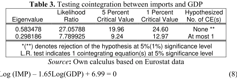
Table 3 presents the results for the cointegration test applied for imports and GDP. Again, one cointegration relation exists (eq. 8).

Table 3. Testing cointegration between imports and GDP

Likelihood 5 Percent 1 Percent Hypothesized Eigenvalue Ratio Critical Value Critical Value No. of CE(s)

0.583478 27.05788 19.96 24.60 None ** 0.298186 7.789925 9.24 12.97 At most 1 *(**) denotes rejection of the hypothesis at 5%(1%) significance level L.R. test indicates 1 cointegrating equation(s) at 5% significance level

Source: Own calculus based on Eurostat data

Log (IMP) – 1.65Log(GDP) + 6.99 = 0 (8)

Table 4 presents the results for the trivariate stochastic system composed of exports, imports and GDP. One cointegration relation consisting on all 3 variables was identifier. This equation might be substituted by a system of two related equations, on only two variables (see eq. 9 and 10)

Table 4. Testing cointegration relation between GDP, exports and imports

Likelihood 5 Percent 1 Percent Hypothesized Eigenvalue Ratio Critical Value Critical Value No. of CE(s)

0.958330 94.21684 34.91 41.07 None ** 0.565677 24.30125 19.96 24.60 At most 1 *

0.237105 5.953962 9.24 12.97 At most 2 *(**) denotes rejection of the hypothesis at 5%(1%) significance level L.R. test indicates 2 cointegrating equation(s) at 5% significance level

Source: Own calculus based on Eurostat data

Log (GDP) = 0.34 Log (Exp) + 0.27 Log (Imp) + 4.11 (9)

Log(GDP) = 0.88 Log(Imp) + 1.71

Log(EXP) =1.77 Log(Imp) + 7.009 (10)

The previous relations are extremely important, as the obtained coefficients permit us to comment the results. In equation 9 we obtained a higher coefficient for exports (0.34) than the import coefficient (0.27). This means that the weight of exports in the long term equilibrium relation is higher than the weight of imports. The cointegration relations demonstrate that the GDP, exports and imports have a similar trend all of them, this means that it is assumed that they evolve towards equilibrium on long term. Of course, the obtained results stimulate us to test the causality, because by the fact that they tend towards equilibrium on long term it doesn’t mean that it exists a causal relation between them. The following step in our methodology is to test the causality, considering the cointegration results that we obtained. We have to estimate a representation of VECM kind for the causality tests.

Step 3. The study of Granger causality

The econometric software Eviews implements the Granger causality tests by applying the Wald test over the coefficients of a system represented in VAR type, as we described them previously. The VAR representation from equation (2) can be rewritten under the following form:

p t p t

p t p t

t y y x x

y =α₀ +α_{1 −1} +...+α ₋ +β_{1 −1}+...+β ₋ (11) In this equation, the Wald test assumes the testing of the restriction:

0 ...

2

1 =β = =βp =

β (12)

In order to obtain the representation of type VECM, we must estimate a VAR model in Eviews in which we must include the specific elements cointegration equations (eq. 13). Wald tests are applied on the coefficients of these equations.

p t p t

p t p t

t c y x y y x x

y = + + ∇ ₋ + + ∇ ₋ + ∇ ₋ + + ∇ ₋

∇ α₀ γ₀ ( , ) α_{1 1} ... α β_{1 1} ... β (13) Table 5 presents the Wald tests applied for Granger causality in the case of Exports and GDP. The first hypothesis due to which exports do not cause economic growth is accepted, being given the high value of probability. The second hypothesis, GDP does not Granger cause exports is rejected, being given the low level of probability (under 5%). In other words, the econometric test demonstrates that we do not have sufficient evidences for situating ourselves in the conditions in which exports represent a determinant of economic growth. The relation is valid vice versa, considering the second conclusion, which rejects the null hypothesis of non-causality on the relation GDP-exports.

Table 6 presents the conclusions of the Granger tests on imports.

Table 5. The Wald tests in the VECM model between exports and GDP

Null Hypothesis Obs F-Statistic Probability

LOG_EXP does not Granger cause LOG_GDP 21 0.63046 0.6494 LOG_GDP does not Granger cause LOG_EXP 12.036 0.00026

Source: Own calculus based on Eurostat data

Table 6. The Wald tests in the VECM model between imports and GDP

Null Hypothesis Obs F-Statistic Probability

LOG_IMP does not Granger cause LOG_GDP 21 0.9758 0.4538 LOG_GDP does not Granger cause LOG_IMP 2.2984 0.1141

Source: Own calculus based on Eurostat data (www.eurostat.org)

In both situations, it is accepted the non-causality hypothesis, because the acceptance probability is over the level of 5%. We observe that the probability of accepting the hypothesis “GDP does not cause imports” is lower than in the case of imports does not cause GDP.

After testing the causality on the bivariate model we can draw the can draw the conclusion that in Romania the information about GDP is useful in determining the forecast of exports. Information regarding imports does not allow us to obtain a better prediction of the growth.

the block EU 25 for the causality tests, for reasons of comparability and for seeing how the adhesion of the ten countries affects the causality (in case this will be identified). In tables we will include the results that we had already obtained in the case of Romania. We will complete our analysis also with a trivariate analysis, in order to see if the causality is still kept if we add a third variable, named auxiliary variable. In our case, it is of interest the study of causality exports-GDP, in the presence of imports. Even the imports are not in a causality relationship with GDP, they can affect the causality exports-GDP.

5. A comparative study: Romania, its neighbor countries, EU 15 and

EU 25

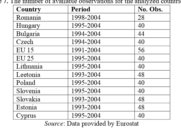
In this section, the same methodology is applied on some countries which present similarities with Romania from the point of view of the economic structure. We will use as reference the groups of EU 15 and EU 25 in order to identify at union level how the adhesion of 10 countries affected the relationship between trade and economic growth. In this way, we want to validate the study for the case of Romania. Table 7 contains information which refers to the number of available statistical observations on each country. We intended to collect a number of observations as high as possible, for a similar period with the one considered for the Romania’s case. The table contains information regarding Romania; during this section Romania’s data will stand near the results obtained on the other countries, for the reason of comparability.

Table 7. The number of available observations for the analyzed countries Country Period No. Obs.

Romania 1998-2004 28

Hungary 1995-2004 40 Bulgaria 1994-2004 44 Czech 1994-2004 40

EU 15 1991-2004 56

EU 25 1995-2004 40

Lithuania 1995-2004 40

Leetonia 1993-2004 48 Poland 1995-2004 40 Slovenia 1995-2004 40 Slovakia 1993-2004 48 Estonia 1993-2004 48 Cyprus 1995-2004 40

Source: Data provided by Eurostat

The methodology of section 3 is applied. Table 8 contains the results obtained by applying the ADF unit root tests.

all series. The same number of the unit roots signifies the fact that the series has, in some way, similar properties, but to see if they tend to equilibrium on long term the cointegration should be tested. The results for of the unit root tests are important as they gives us a clue about the testing of cointegration, which could not be possible if the series had no unit roots.

Table 8. Unit root tests for different developing countries in Central and East Europe

Initial series First

difference

second difference

Slovakia –GDP -0.2954 -2.9406 One unit root

Slovakia – Exp. -0.4289 -3.9633 One unit root

Slovakia – Imp -0.3698 -3.3832 One unit root

Slovenia – GDP -1.1795 -2.9388 -4.5882 Two unit roots

Slovenia – Exp -0.4982 -2.8526 -3.5336 Two unit roots Slovenia – Imp -0.1496 -2.4742 -4.6198 Two unit roots Poland– GDP -1.2731 -1.6639 -2.4379 At least 2 unit r.

Poland – Exp -0.1115 -3.4025 One unit root

Poland – Imp -1.2958 -2.9452 -3.4301 Two unit roots

Leetonia – GDP -0.6896 -4.0783 One unit root

Leetonia – Exp -1.0693 -3.2787 One unit root

Leetonia – Imp -1.1637 -2.6386 -4.6960 Two unit roots

Bulgaria – GDP -1.2121 -3.9434 One unit root

Bulgaria – Exp -0.3792 -3.6152 One unit root

Bulgaria – Imp -0.1024 -3.6149 One unit root

Hungary –GDP -0.3416 -2.3782 -3.2882 Two unit roots

Hungary – Exp -1.4127 -2.6442 -3.2683 Two unit roots Hungary – Imp -2.3520 -2.3985 -3.7786 Two unit roots

Cyprus – GDP -0.9722 -2.7046 -5.3294 Two unit roots

Cyprus – Exp -0.9167 -2.3694 -5.2705 Two unit roots Cyprus – Imp -0.7195 -2.1355 -4.9762 Two unit roots Lithuania –GDP -1.6533 -1.8940 -3.1925 Two unit roots Lithuania – Exp -0.8361 -2.2122 -2.4120 at least 2 unit r. Lithuania – Imp -1.2041 -2.2921 -3.1650 Two unit roots

Czech – GDP -0.3450 -4.1622 One unit root

Czech – Exp -0.0901 -3.2782 One unit root

Czech – Imp -0.0448 -2.3866 -3.4837 Two unit roots Estonia – GDP -2.8697 -2.1187 -4.4131 Two unit roots

Estonia – Exp -1.3507 -3.2980 One unit root

Estonia – Imp -1.2099 -3.3071 One unit root

Romania – GDP -0.8019 -3.0812 One unit root

Romania – Exp -2.7331 -2.5749 -2.9041 At least 2 unit r. Romania – Imp -1.5287 -2.6584 -2.0164 At least 2 unit r.

EU 25 – GDP -1.8538 -3.0869 One unit root

EU 25 – Exp -1.5104 -3.3842 One unit root

UE 25 – Imp -1.3742 -3.3380 One unit root

UE 15 – GDP 0.3436 -3.5440 One unit root

UE 15 – Exp -0.6925 -3.7798 One unit root

Table 9. The cointegration tests

Coefficients of the cointegration relation

No. of

cointegration

relations ( ) Log

(GDP)

1

a ( ) Log

(Exp)

2

a ( ) Log

(Imp)

3

a ( ) Free

term

0 a

Slovakia, GDP, Exp 0

Slovakia, GDP, Imp 0

Slovakia GDP, Exp, Imp 0

Slovenia, GDP, Exp 2 - stationarity Slovenia, GDP, Imp 1 1 -0.7837 -2.4187 Slovenia, GDP, Exp, Imp 1 1 -0.27246 -0.52879 -2.2113

Poland, GDP, Exp 0

Poland, GDP, Imp 0

Poland, GDP, Exp, Imp 1 1 2.274 -5.4680 20.2819 Leetonia, GDP, Exp 1 1 -1.0296 -0.67608

Leetonia, GDP, Imp 0

Leetonia, GDP, Exp, Imp 1 1 -1.6699 0.5621 -0.2894

Bulgaria, GDP, Exp 0

Bulgaria, GDP, Imp 1 1 -0.6802 -2.9267 Bulgaria, GDP, Exp, Imp 1 1 1.05761 -1.5452 -4.3425

Hungary, GDP, Exp 0

Hungary, GDP, Imp 0

Hungary, GDP, Exp, Imp 1 1 -19.0704 16.8459 10.0454

Cyprus, GDP, Exp 0

Cyprus, GDP, Imp 1 1 -1.191 0.9983 Cyprus, GDP, Exp, Imp 0

Lithuania, GDP, Exp 0

Lithuania, GDP, Imp 1 1 -0.4708 -4.8073 Lithuania, GDP, Exp, Imp 1 1 1.07738 -2.0027 -1.0916

Czech, GDP, Exp 0

GDP, Imp 1 1 -0.7371 -2.9130

Czech, GDP, Exp, Imp 1 1 1.3094 -2.1664 -1.6955 Estonia, GDP, Exp 2 – stationarity Estonia, GDP, Imp 2 – stationarity Estonia, GDP, Exp, Imp 2 1 -1.2409 1.7864

1 -0.07665 -7.21926

Romania, GDP, Exp 1 1 -0.6266 -4.1422 Romania, GDP, Imp 1 1 -0.6034 -4.2215 Romania, GDP, Exp, Imp 2 1 -0.88838 -1.7163

1 -1.7753 7.0095

EU 25, GDP, Exp 0 EU 25, GDP, Imp 0 EU 25, GDP, Exp, Imp 0 EU 15, GDP, Exp 0 EU 15, GDP, Imp 0

EU 15, GDP, Exp, Imp 2 1 -0.58484 -6.7501

1 -0.96488 -0.5025

Source: Own calculus based on Eurostat data

0 3

2 1

0 +a LogGDP+a LogEXP+a LogIMP=

a (14)

The inexistence of cointegration for some countries (Slovakia, Poland, Hungary, Cyprus, EU 25 and EU15) determines the application of the autoregressive model of type VAR on the differentiated process (VARD), according with the methodological developments presented in section 3 (see figure 1).

In the case of identifying stationarity2 (Slovenia Exp-GDP, Estonia Exp-GDP, Imp-GDP), we will apply the VAR model on the levels data (VARL).

In case of identifying a cointegration relation, we will apply the VECM model. The coefficients of the cointegration relations reflect the weight of the variables in the equilibrium long term relation. For example, in the case of Slovenia we identified one cointegration relation between GDP and imports which corresponds to the following equation:

Log(GDP)=0.7837 Log (Imp)+2.4187 (15) In three cases, Slovenia (GDP, exports), Estonia (GDP, exports), Estonia (GDP, imports), we identified stationarity. This means that the type of the employed representation for the models will be VARL, respectively we will use the initial series, without differentiation. In most cases, a cointegration relation was obtained which means that we can apply the Wald test over the coefficients on the VECM model.

Table 10 contains the results of the Granger-causality tests for the models containing GDP and Exports. Model type represents the kind of model on which the testing was performed and F value is the computer F statistics for the Wald test. The table contains the probability inferred for the acceptance of the null hypothesis: “Exports does not Granger-cause GDP”. The significance level is 5%.

Table 10. Bivariate models, GDP expressed as function of exports

Model type Value F Prob. Conclusion

Slovakia VARD 2.6014 0.0532 Exp doesn’t cause Granger GDP Slovenia VARL 2.1183 0.1060 Exp doesn’t cause Granger GDP Poland VARD 0.9116 0.4718 Exp doesn’t cause Granger GDP Leetonia VECM 2.1826 0.0918 Exp doesn’t cause Granger GDP Bulgaria VARD 3.3483 0.0221 Exp causes Granger GDP

Hungarian VARD 1.1458 0.3571 Exp doesn’t cause Granger GDP Cyprus VARD 2.3330 0.0834 Exp doesn’t cause Granger GDP Lithuania VARD 2.6577 0.0553 Exp doesn’t cause Granger GDP Czech VARD 3.5122 0.0202 Exp causes Granger GDP

Estonia VARL 1.2184 0.3205 Exp doesn’t cause Granger GDP Romania VECM 0.63046 0.6494 Exp doesn’t cause Granger GDP UE 25 VARD 1.14035 0.3595 Exp doesn’t cause Granger GDP UE 15 VARD 3.3585 0.0179 Exp causes Granger GDP

Source: Own calculus based on Eurostat data

We can notice that a direct ELG relationship can be inferred only on 3 cases: Czech Republic, Bulgaria and EU15. For EU 15 we expected this result, as literature proved that ELG is valid for the most important countries of EU, from the economic point of view (Germany, UK, France). The only surprising result is the one of Bulgaria,

2

while the Czech Republic was considered during last 10 years on the top of the ascending countries with respect to its economic performance.

We tried to introduce the imports as the third variable of the model, keeping GDP as the dependent variable. Table 11 presents the results.

Table 11: Trivariate Models, GDP expressed as function of exports, in the presence of imports

Model type Value F Prob. Conclusion

Slovakia VARD 2.2309 0.08930 Exp does not cause Granger GDP Slovenia VECM 0.5812 0.67937 Exp does not cause Granger GDP Poland VECM 1.4726 0.24445 Exp does not cause Granger GDP Leetonia VECM 1.4899 0.23007 Exp does not cause Granger GDP Bulgaria VECM 4.4447 0.00717 Exp causes Granger GDP

Hungary VECM 1.1871 0.34402 Exp does not cause Granger GDP Cyprus VARD 1.2375 0.32534 Exp does not cause Granger GDP Lithuania VECM 4.2140 0.01106 Exp causes Granger GDP

Czech VECM 3.4708 0.02418 Exp causes Granger GDP

Estonia VECM 0.2556 0.90381 Exp does not cause Granger GDP Romania VECM 1.98104 0.19048 Exp does not cause Granger GDP EU 25 VARD 0.82856 0.52125 Exp does not cause Granger GDP EU 15 VECM 0.49774 0.73746 Exp does not cause Granger GDP

Source: Own calculus based on Eurostat data

We can notice that only for the case of Lithuania the inclusion of imports changed the results. We can conclude that imports are not too relevant with respect to their influence in the relationship between exports and GDP, in the case of ELG testing.

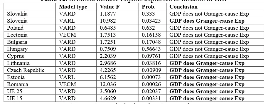
Table 12 contains the results for testing the GLE relationship, on bivariate models.

Table 12. Bivariate models. Exports expressed as function of GDP

Model type Value F Prob. Conclusion

Slovakia VARD 1.1877 0.333 GDP does not Granger-cause Exp Slovenia VARL 10.982 0.03425 GDP does Granger-cause Exp

Poland VARD 0.6485 0.632 GDP does not Granger-cause Exp Leetonia VECM 1.7513 0.16158 GDP does not Granger-cause Exp Bulgaria VARD 1.7251 0.17048 GDP does not Granger-cause Exp Hungary VARD 0.7509 0.56643 GDP does not Granger-cause Exp Cyprus VARD 2.2039 0.09761 GDP does not Granger-cause Exp Lithuania VARD 2.9686 0.03816 GDP does Granger-cause Exp

Czech Republic VARD 4.2265 0.00909 GDP does Granger-cause Exp

Estonia VARL 6.1562 0.00073 GDP does Granger-cause Exp

Romania VECM 12.036 0.00026 GDP does Granger-cause Exp

UE 25 VARD 3.5060 0.02037 GDP does Granger-cause Exp

UE 15 VARD 4.6629 0.00331 GDP does Granger-cause Exp

Source: Own calculus based on Eurostat data

We can notice that more countries exhibit an inverse GLE relationship. Only on the case of Czech Republic and EU 15 both ELG and LGE relationships are valid.

the idea that the imports determine that the information about GDP is relevant in the predictability of exports. It can be concluded that in Hungary and Cyprus it exists an interdependent relation.

Out of this analysis we can conclude that the most important relationship to be tested is the one between exports and GDP, while imports might influence this relationship in an unexpected way.

Table 13. Trivariate models, Exports as Function of GDP, in the presence of imports

Model type Value F Prob. Conclusion Slovakia VARD 0.6924 0.6030 GDP doesn’t cause Granger Exp Slovenia VECM 2.8528 0.0479 GDP causes Granger Exp

Poland VECM 1.1430 0.3624 GDP doesn’t cause Granger Exp Leetonia VECM 1.20905 0.3275 GDP doesn’t cause Granger Exp Bulgaria VECM 0.78190 0.5472 GDP doesn’t cause Granger Exp Hungary VECM 4.86016 0.00581 GDP causes Granger Exp

Cyprus VARD 4.25860 0.01115 GDP causes Granger Exp

Lithuania VECM 1.16753 0.35210 GDP doesn’t cause Granger Exp Czech Republic VECM 2.10275 0.1148 GDP doesn’t cause Granger Exp Estonia VECM 3.73691 0.0143 GDP causes Granger Exp

Romania VECM 10.4442 0.0029 GDP causes Granger Exp

EU 25 VARD 3.08646 0.0368 GDP causes Granger Exp

EU 15 VECM 5.85392 0.0009 GDP causes Granger Exp

Source: Own calculus based on Eurostat data

6. Conclusions

In this article, we analyzed econometrically the relation between foreign trade and economic growth in Romania, on a period during 1998-2004, using quarterly data. We used the vales of the indicators expressed in Euro. The econometric findings showed us that in Romania exports do not cause Granger GDP. Inversely, we found out that GDP causes Granger exports, in other words that the information about GDP presents importance in what exports are concerned. More than that, the relation between imports and GDP from a causal point of view did not verify. What does it mean this thing? It is a good or a bad one? These are a few questions at which we will try to answer.

The fact that GDP causes exports suggests that the greater the GDP is the surplus is dedicated to stimulate the production of goods addressed to the internal consumers but also to the foreign ones.

In the Romania’s case, the problem is that the actual structure of exports proved to be not capable of generating a feed-back ELG relation. This means that exports do not bring enough value added for providing relevant information of GDP.

In fact, during the last years, in Romania we assisted at an economic growth based mainly on consumption. An important part of the consumption is based on imports. So, an import based on the final consumption cannot constitute the relevant information referring to the economic growth of the country, as the trivariate model of GDP expressed in function of exports proved.

is to obtain Granger causality evidence between trade and growth. The relative disordered and unpredictable character of the economic activity in Romania and the lack of stabilization during the considered period can be possible explanations of the unfavourable results that we obtained when we tested ELG. The above-mentioned conclusion of Marin [1992] is emphasized by our findings that ELG holds for EU15, Czech Republic and Bulgaria. EU15 is a well-recognized economic power of the World; Czech Republic is a small country with the best economic performances out of the 10 countries that adhered to EU, while for the case of Bulgaria, the presence of the Monetary Council might assure an ordered character of the economic activity.

Our conclusions are not so pessimistic for Romania, if we see them in the context of the comparison with the neighbor countries, with those which joined EU and with Bulgaria, which intends to join. We saw that after applying our study methodology, only one single country verified double-sense causality and that is Czech Republic. The remaining countries have situations which can not be analyzed in a generic framework; one should look carefully from case to case. More, as we consider EU as a whole with 25 countries, the ELG relationship does not remain valid, while GLE comes into attention.

Adding imports to the bivariate models between exports and GDP did not change too much the ELG results. Only in Lithuania the ELG relationship was validated only in the presence of imports. This might express evidence that imports could be especially technology intensive, and they contributed to the technology-intensive goods export which stimulated also the economic growth.

The inverse relation (GDP cause exports) was validated also in the presence of imports in countries like Slovenia, Estonia, Romania, EU 25 and EU 15. Hungary and Cyprus are two countries for which we obtained that GDP causes Granger exports but only in the presence of imports. This means that in these countries a very strong relationship between exports and imports might exist.

Further studies concerning the trade specialization for the Romania’s case should be performed. Determining how the country’s trade specialization evolved from 1990 till now might reveal why ELG was not identified and could reveal useful insights for trade policy makers.

References

1. Andrei, Tudorel, Statistics and Econometrics, Ed. Economică, Bucureşti, 2003 (in Romanian)

2. Axfentiou, P. C.; Serletis, A., Exports and GNP causality in the industrial countries 1950-1985, Kyklos 44, 1991, p. 167-179

3. Balassa, Bela, Exports, Policy Choices and Economic Growth in Developing Countries after the 1973 Oil Schock, Journal of Development Economics, 18: 23-35,1985

4. Box, G., Jenkings, G. Reinsel G., Time Series Analysis-Forecasting and Control, Prentice Hall, 1994

5. Bresson, G., Pirotte, A., Econometries des series temporelles, PUF, Paris, 1995

7. Dominiguez, Loreto, Economic Growth and Import Requirements, Journal of Development Studies, 6(3), p.283-299, 1970

8. Engle, R.F., Granger, C.W.J. Cointegration and error correction: representation, estimation and testing. Econometrica 55, 251-76, 1987.

9. Feder, Gerhson, On Exports and Economic Growth, Journal of Development Economics, 12, p.59-73, 1983

10.Florea, I., (coord.). I Parpucea, A. Buiga, D. Lazăr, Inteferential Statistics, Presa Universitară Clujeană, 2000 (in Romanian)

11.Giles, J.A., Williams C.L., Export-Led Growth: A Survey of the Empirical Literature and Some Noncausality Results, Part 1, Journal of International Trade and Economic Development, 2000, 9, p. 261-337

12.Grossman, G.E., Helpman , Innovation and Growth in the Global Economy, Cambridge Mass.: MIT Press, 1991

13.Johansen, S. Statistical analysis of cointegration vectors. Journal of Economic Dynamics and Control 12, 231-54, 1988.

14.Jung, W. S., Marshall, P. J., Exports, Growth and Causality in Developing Countrie, Journal of Development Economics, February 1985, 1-12.

15.Kavoussi, R. M, International Trade and Economic Development: the Recent Experience of Developing Countries, in Journal of Developing Areas, no.19, pp.379-392, 1985

16.Krugman, Paul; Helpman,E., Imperfect Competition and International Trade: Evidence from fourteen Industrial Countries, Cambridge: Harvard University Press, p.28, 1988

17.Larre, B., Torres, R., La convergence est-elle spontanee? Experience comparee de l’Espagne, du Portugal et de la Greece, Revue Economique de l’OCDE, no.16, Printemps, p.193-223,1991

18.Marin, D., Is the Export-led Hypothesis Valid for Industrialized Countries?, Review of Economics and Statistics, 74, 1992, p.678-688

19.Michaely , Michael, Exports and Growth: an empirical investigation, Journal of Development Economics, 4, p.49-53, 1977

20.Perreira, A., Importacao de bens de capital e evolucao economica interna: os casos da Grecia e de Portugal, Banco de Portugal, Boletim Economico, December, p. 59-66, 1996

21.Pop-Silaghi, Monica, Measuring trade performance of Romania, in Proceedings of the conference: “The Impact of European Integration on the National Economy”, 28-29 October, Faculty of Economics, Babes-Bolyai University, Cluj-Napoca, 2005 22.Tyler, William, Growth and Export Expansion in Developing Countries, Journal of