A Predictive Traffic Analysis on a General Purpose Heterogenous Distributed Network

A Predictive Traffic Analysis on a General Purpose

Heterogenous Distributed Network

Sharmi S

Research Scholar, MS University, India

M. Punithavalli

SREC, India

Munesh Singh Chauhan

University India

ABSTRACT

In this paper, a new approach is proposed to predict the fractal behavior of a distributed network traffic. In this research, traffic traces are collected from a distributed network operated by NETRESEC an independent software vendor with focus on the network security field, network forensics and analysis of network traffic. A traffic analysis on packet, connection, protocol and application layers are taken into consideration. Apart from it, an investigation of self-similar and long-range dependent behavioral characteristic is made prior to the collection of traffic traces. Traffic prediction plays an important role in guaranteeing Quality of Service (QoS) in distributed networks due to the diversity of services in a real-time network application. Traffic prediction can be useful for dynamic routing, congestion control and prevention, autonomous traffic engineering, proactive management of the network etc. The forecasting methods can be broadly classified into two categories: linear prediction and nonlinear prediction models. Hence, the idea behind this research is to propose a Multiple Regression-booster equation based on the correlation structure to have a more accurate predicted traffic data result than using the later nonlinear prediction models involving Neural Networks. The traffic is sniffed and exported to NeuroSolutions builder, SPSS and then examined. Further, the exported and dissected traffic data is fed as input to train the neural network to let it predict the resultant fractal behavior of the distributed network traffic and an equation is proposed to derive the ultimate close network traffic prediction in SPSS.

Keywords

Fractal behavior, sniffing, predict, SPSS, NeuroSolution builder, predictor.

1.

INTRODUCTION

For the examination of local problems in a small network, monitoring at a single observation point is sufficient to train the network builder. In such cases, a network analyzer may be used which can be a machine running Wireshark and is directly connected to a network segment or the monitoring port of a switch or a router. In larger networks, it is often necessary to perform simultaneous monitoring at multiple observation points to train the constructed neural network in a more efficient manner.

In this research a Neural Network (Multilayer Perceptron) is proposed to be used to predict the dependent variable values over different independent variable value distributions using two specific modeling tools, viz., SPSS and NeuroSolutions. One objective of this is to find the effect of the dependent variable values distributions in the dataset using different

modeling tools in the Neural Network prediction performance. A second objective is to compare the performance of the two modeling tools in the prediction of the dependent variable values.

Network traffic measurement and analysis are important for better understanding of the network behavior. In this research, collected traffic traces from a distributed network operated by NETRESEC an independent software vendor with focus on the network security field, network forensics and analysis of network traffic is being used. The performed traffic analysis on packet, connection, protocol, and application layer. Investigation of self-similar and long-range dependent characteristics of the collected traffic traces are employed using various estimators.

The relative fitness of various Predictive functions was investigated. The conclusion is made as the proposed equation is ideal to have a more accurate result than SPSS , NeuroSolutions, Neural predictor respectively.

2.

TRAFFIC

COLLECTION

AND

CHARACTERIZATION

There are many traffic collection programs available. Many previous traffic traces were collected using the Wireshark. Several analysis tools for Wireshark traces exist. Hence, Wireshark is chosen as the traffic collecting tool. Wireshark implements a range of filters that facilitate the definition of search criteria and currently supports over 1100 protocols.

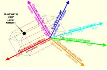
Fig 1: Heterogeneous distributed network space diversity (Yongguang Zhang 2000)

router operating systems, etc.) into a multidimensional space. Each network element that instantiates a functional capability is represented as a point along the dimension. It also also illustrates an example of such diversity space. where, UDP, RTP and TCP are the three network elements along the dimension of transport protocols, while satellite, wireless, and fiber-optic networks are examples of elements for the communication medium (or physical network connectivity) (Yongguang Zhang 2000).

The given diversity space diagram of heterogeneous networks helps us to inspect the traffic and dissect it based on certain parameters such as protocols, bandwidth, Pareto-distribution etc. The network traffic behavior falls within the classified two regions, short-range dependencies (SRD) and long-range dependence (LRD). The physical mechanisms that control the two regions are clearly identified and generalized by six factors: bandwidth, delay, number of connections, packet sizes, TCP window sizes and Pareto shape factor. The software sniffer “Wireshark” (open source protocol analyzer) is used to capture a live traffic from the network or can also work on a captured traffic (NETRESEC) to analyze the traffic based on customized protocol classification. The captured .Cap (packet capture) file is exported as .Csv format.

3. ESTIMATING TRAFFIC ON ANN

PREDICTOR MODEL

A Neural Network (Multi-layer Perceptron) is proposed to be used to predict the dependent variable values over different independent variable value distributions using NeuroSolutions. Genetic algorithms are combined with neural networks to enhance their performance by taking some of the guesswork out of optimally choosing neural network parameters, inputs etc. In general, genetic algorithms can be used in conjunction with neural networks in the following four ways. It is to be used to choose the best inputs to the neural network, optimize the neural network parameters (such as the learning rates, number of hidden layer processing elements, etc.), train the actual network weights (rather than using back propagation), or to choose/modify the neural network architecture. In each of these cases, the neural network error is the fitness used to rank the potential solutions.

It is a computational method motivated by biological models. ANNs attempt to mimic the fundamental operation of the human brain and can be used to solve a broad variety of problems [6]. One of the most important features of ANNs is that it can discover hidden patterns from data sets [7], and solve complex problems especially when a mathematical model does not exist (or when the model is not suitable for the case at hand). Furthermore, ANNs are commonly immune to noise and irregularities present in the data [8, 9]. ANN learning is typically based on two data sets: the training set and the validation set. The training set is used on a new artificial neural network, as its name indicates, for training. The validation set is used after the neural network has been trained to assess its performance. The validation set in most cases is similar to the training set but not same [10, 11].

4.

DATA MAPPING – ANN

In artificial intelligence, a desired output is commonly known as the target. For the specific case of ANNs, the target is used for network training [5]. ANNs can map a given input to a desired output; when an ANN is used for this purpose, the ANN is typically called a mapping ANN. The network is

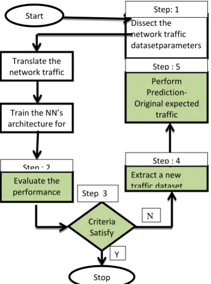
trained by applying the desired input to the ANN, and then monitoring the actual ANN output. The difference between the actual ANN output and the desired output is normally used to manage the learning process. During the process of training, the learning algorithm attempts to reduce the error measured between the actual network output and the targeting the training set [5, 7]. The training process may be time consuming, but when the process has been successfully completed, an ANN can quickly calculate its output once the input data has been applied to the network input. The Flow diagram for prediction using NeuroSolutions is shown in figure 2.

5.

DATA CLASSIFICATION

Data classification or just classification is the process of identifying an object from a set of possible outcomes [5, 8]. An ANN can be trained to identify and classify any kind of objects. These objects can be numbers, images, sounds, signals, etc. An ANN used for this purpose is also known as a classifier.

The traffic data is trained initially with a network traffic-dataset that had been downloaded from wireshark sample captures as a pcap file and the data is exported to network builder for prediction. The predicted fractal behavior on the traffic data set is shown in table 1 in the appendix.

Fig 2 : Flow diagram for prediction using NeuroSolutions

6.

INVESTIGATION

On investigating the effect of dependent variable values and the distribution on the prediction accuracy rate. The results of the analyses lets us to find the effect of the dependent variable values distribution on prediction accuracy that exploits and leads us generating an equation that would predict the expected traffic based on the independent variable-values distribution using the modeling tool SPSS.

Start

Translate the network traffic

data parameters.

Train the NN’s architecture for

N number of epochs.

Evaluate the performance

Criteria Satisfy

Extract a new traffic dataset dissected accordingly

Perform Prediction- Original expected

traffic Dissect the network traffic datasetparameters

Stop

Step: 1

Step : 2

Step 3

Step : 4 Step : 5

Correlation Coefficient, R, is a measure of the strength of the association between the independent (explanatory) variables and the dependent (prediction) variable.Ris never a negative value. This can be seen from the formula below, since the square root of this value indicates the positive root[2,3].The most common formula for computing a product-moment correlation coefficient (r) is given below.The correlation (r) between two variables is:

Where Σ is the summation symbol, x = xi - x, xi is the x value for observation i, x is the mean x value, y = yi - y, yi is the y value for observation i, and y is the mean y value. The coefficient of multiple correlation estimates the combined influence of two or more variables on the observed (dependent) variable. To analyze the traffic data using multiple regression, part of the process involves the following assumptions to be verified[8].

To analyze the traffic data using multiple regression, part of the process involves the following assumptions to be verified.

 The dependent variable is measured on a continuous scale.

 Two or more independent variables, are continuous or categorical.

 Observations should be recorded.

 Linear relationship exists between the dependent variable and each of the independent variables.

 Traffic data shows homoscedasticity, which is where the variances along the line of best-fit remain similar as one move along the line.

 The data does not show multicollinearity, which occurs when two or more independent variables are highly correlated.

 There are no significant outliers, high leverage points or highly influential points.

 Residuals (errors) are approximately normally distributed.

When the above listed assumptions are not violated, the Multiple Correlation Coefficient (R), is computed to measure the strength of the association between the independent (explanatory) variables and a single dependent (prediction) variable. The initial footstep to predict the network traffic leads the way to exploit the correlation structure further to probe into the degree of association between the predictor variable (dependent) and the other independent variables.

7.

MULTIPLE

REGRESSION

EQUATION BOOSTER PREDICTION

PHASES

In MR-Booster, by using each feature of the association existing between the actual traffic and the dissected traffic explicitly helped to generate the prediction equation and the standard error factor when probed in further boosts a better way to refine the regression equation that predicts the network traffic. The correlation structure of traffic is finally generated in a much easier way.

Phase 1

The sniffed traffic data are plotted as a scatter plot graph to visualize if there is a possible linear relationship.

Calculate and interpret the linear correlation coefficient, using the data sets.

Phase 2

Determine all possible regression equation for the data by refining it further by adjusting the constant standard error from it.

Select and apply the best generated regression equation and forecast.

Phase 3

Identify outliers and note the observations.

Process and interpret the performance of MR-booster prediction.

Table 1 Correlation Coefficient for the Training Dataset

Correlation

Co-efficient Datasets

0.988 MR1(y):(X1,X3)

0.953 MR2(y):(X1,X2)

0.904 MR3(y):(X2,X3)

0.940 Average (r)

The correlation coefficient is 0.940. This value of r suggests a strong positive linear correlation since the value is negative and close to 1. Since the above value of r suggests a strong positive linear correlation, the data points should be clustered closely about a positively sloping regression line. A strong positive linear relationship between actual traffic and filtered traffic via the transport protocols is visualized (seen) in table 3, this leads further more close to the linear regression analysis (y).

COMPUTE y = 1 * x1 + 1 * x2 - 0. EXECUTE.

8.

IMPORTANCE OF INDEPENDENT

VARIABLES

IN

MULTIPLE

REGRESSION

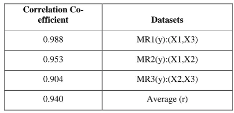
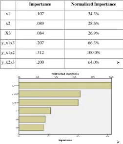
The correlation coefficient also helps the tool to compute the importance, which is shown in the Table 2 and the pictorial representation is depicted as shown in Fig 3.

Table 2 Independent Variable Importance

Importance Normalized Importance

x1 .107 34.3%

x2 .089 28.6%

X3 .084 26.9%

y_x1x3 .207 66.3%

Importance Normalized Importance

x1 .107 34.3%

x2 .089 28.6%

X3 .084 26.9%

y_x1x3 .207 66.3%

y_x1x2 .312 100.0%

y_x2x3 .200 64.0%

Fig 3: Independent variable importance graph.

9.

PERFORMANCE METRICS

Error metrics are the mathematical equations which are used to describe an error between actual and predicted values. The difference between actual and predicted values shows how well the model has performed. The main idea of forecasting techniques is to minimize this value, since this should influence the performance and reliability of the model. These error metrics have significant importance in forecasting th future, as the measurements taken by these metrics highly influence the future planning.

According to Bryan (2005), any metric which measures the error should have five basic qualities which are: validity, easy to interpret, reliability, presentable and have statistical equation (i.e. can be represented in the form of mathematical equation). Here validity refers to the degree to which an error metric measures what it claims to measure. In other words, validity refers to whether error metric really measures what it intend to measure. The metric should measure the results which can relate to the available data. Validity also refers to the authenticity of the measurement.

Easy to Interpret refers to the simplicity of the metric. The metric should be easy to understand and avoid complexity. The practitioners normally avoid using complex metrics since especially financial forecasting is complex and there is a need to be able to explain and motivate decisions, which is easier if the metric is simple and easy to understand.

Reliability is the consistency of the error metric to measure error using the same measurement method on same subject. If repeated measurements are taken and every time the results are highly consistent or even identical then there is a high degree of reliability, but if the measurements have large variations then reliability is low. The error metric is reliable when it is evident that it will produce the same result every time it is given the same data.

Presentable refers to the ability of error metric and its measurement to be represented in a form which is easy to understand.

The statistical equation suggests that the error metric can be represented in the form of mathematical equations. Mathematical equations are most common and easy to interpret form of error metrics.

On the basis of reliability, validity and wide use, the following performance (error) measuring metrics are recommended for evaluating models.

 Mean Square Error

MSE (Mean Square Error) is a scale dependent metric which quantifies the difference between the forecasted values and the actual values of the quantity being predicted by computing the average sum of squared errors.

The MSE for the predictor traffic by Neural Networks and the actual traffic is 0.004 and the MSE for the predictor traffic by the generated SPSS booster regression equation and the actual traffic is 0.001. The Neural Network predictor model results are compared using their MSEs as a measure of how well it can explain the set of observations. The unbiased equation predictor model with the smallest MSE is generally interpreted as best explaining the variability in the observations.

 Root Mean Square Error and Normalized Mean Square Error

Root mean Square Error (RMSE) is square root of average of sum-squared errors and is given by following formula:









n

1 i

2 i

i

y

ˆ

)

y

(

n

1

RMSE

where

Ŷi = estimated traffic

yi = actual traffic

n = number of observations There is one problem with RMSE and it is that they may be close to 0 if large positive and negative errors cancel out each other. RMSE gives high weight to the large errors and are generally useful where large errors are not of importance. RMSE are more sensitive than other metrics to the infrequent large errors as the squaring process gives large weight to very

large errors

(Decision 411 2010). NMSE (Normalized Mean Square Error) can be expressed as MSE divided by the variance of the predicted time series.

 Mean Absolute Percentage Error

MAPE (Mean Absolute Percentage Error) is a metric widely used to evaluate the predictions precision. MAPE calculates the prediction error as a percentage of the observed value. Expressed in percentage terms, it presents the advantage of being easy to interpret. Forecast Error is the deviation of the actual from the forecasted traffic.

 Error = absolute value of {(Actual – Forecast) = |(A - F)|

 Error (%) = |(A – F)|/A

The absolute values are taken because the magnitude of the error is more important than the direction of the error. The Forecast Error can be bigger than Actual or Forecast but NOT both. Error above 100% implies a zero forecast accuracy or a very inaccurate forecast.

 Error close to 0% => Increasing forecast accuracy

 Forecast Accuracy is the converse of Error

 Accuracy (%) = 1 – Error (%)

The MAPE is very close to 0% as it is 2% (0.02) and henceforth the forecast accuracy is 0.98%.

 Correlation Coefficient

Coefficient of correlation (r) indicates the degree of association between two variables, being a measure of linear dependence. The linear correlation coefficient is sometimes referred to as the Pearson product - moment correlation coefficient (PMCC) and is defined as: r = COV (Y, ˆY). The absolute value of both the actual traffic and the forecasted traffics Pearson correlation coefficients are less than or equal to 1 which is shown in Table 4. Correlations equal to 1 or -1 correspond to data points lying exactly on a line, or to a bivariate distribution entirely supported on a line (in the case

of the traffic correlation).

The Pearson correlation coefficient is symmetric corr(X,Y) = corr(Y,X). The absolute value for correlation interpretation is listed in Table 3.

Table 3 Absolute Value of Correlation Coefficient Interpretation

0.90 – 1.00 Very High

Correlation 0.70 – 0.89 High Correlation

0.40 – 0.69 Moderate

Correlation 0.20 – 0.39 Low Correlation

0.00 – 0.19 Very Low

Correlation Source: Guide to interpretation of the correlation coefficient (Tersine 1988)

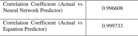
Table 4 Correlation coefficient between the actual and the forecasted traffic

Correlation Coefficient (Actual vs

Neural Network Predictor) 0.996608

Correlation Coefficient (Actual vs

Equation Predictor) 0.999733

 Coefficient Efficiency

Coefficient Efficiency (E): The efficiency coefficient can take values in the domain (−∞, 1]. If E = 1, a perfect fit is had between the observed and the forecasted data. A value of E = 0 occurs when the prediction corresponds to estimating the mean of the actual values. An efficiency less than zero, i.e. −∞ < E < 0, indicates that the average of the actual values is a better predictor than the analyzed forecasting method. The closer E is to 1, the more accurate the prediction is as the coefficient efficiency stays at 0.9 for the forecasted traffic. The major drawback of our solution is that in high-speed networks, the need to restrict the traffic analysis to specific packet streams arises. Otherwise, the amount of monitoring data risks exceeds the available bandwidth between the exporter and the collector, resulting in packet losses or unacceptable high delays. In this respect, distributed network analyzers have the advantage as they only export reports with analysis results which can be much smaller than the examined packet data.

10.

CONCLUSION

The experimental results demonstrates that 1) the regression model is more effective for traffic prediction; and 2) both the proposed prediction equation and standard error based R (correlation coefficient) update scheme are effective to predict the traffic in a easier way.

The goal of the experiments is to evaluate and to compare the performance of the prediction approaches presented in Sections enlisted above. The intention is to identify the best forecasting method for network traffic prediction, taking into account the accuracy but also the complexity of the solutions. To assess the prediction performance, the performance metrics described above are used. In this research, the results of the performance concerning both forecasting methods and error metrics are analyzed. First the relationships between the considered errors matrices (i.e. MAPE, RMSE and MSE) are examined considering the linear correlation between the actual traffic and the forecasting multiple regression equation model.

11.

FUTURE WORK

12.

REFERENCES

[1] Cortez, P., Rio, M., Rocha, M. and Sousa, P. “Internet Traffic Forecasting using Neural Networks”, International Joint Conference on Neural Networks, Vancouver, Canada, pp. 2635 - 2642, 2006.

[2] Li, Z., Wang, R. and Bi, J. “A Multipath Routing Algorithm Based on Traffic Prediction in Wireless Mesh Networks”, Fifth International Conference on Natural Computation, Tianjin, China, Vol. 6, pp. 115-119, August 2009.

[3] Dharmadhikari, V.B. and Gavade, J.D. “An NN Approach for MPEG Video Traffic Prediction”, 2nd International Conference on Software Technology and Engineering, San Juan, USA, pp. V1-57 - V1-61, 2010. [4] Feng, H. and Shu, Y. “Study on Network Traffic

Prediction Techniques, International Conference on Wireless Communications, Networking and Mobile Computing, Wuhan, China, pp. 1041-1044, 2005. [5] Mao, G. “Real-Time Network Traffic Prediction based

on a Multiscale Decomposition”, 4th

International Conference on Networking, Reunion Island, France, Lecture Notes in Computer Science, Vol. 3420, pp. 492-499, 2005.

[6] Dai, J. and Li, J. VBR “MPEG Video Traffic Dynamic Prediction based on the Modeling and Forecast of Time Series, Fifth International Joint Conference on INC, IMS and IDC, pp. 1752-1757, Seoul, Korea, 2009.

[7] Cai, L., Wang, J., Wang, C. and Han, L. “A Novel Forwarding Algorithm over Multipath Network”, International Conference on Computer Design and Applications, pp. V5-353 - V5-357. Qinhuangdao, China, 2010.

[8] Abdennour, “Evaluation of neural network architectures for MPEG-4 video traffic prediction”, IEEE Transactions on Broadcasting, Vol. 52, No. 2, pp. 184-192, 2006. ISSN 0018-9316.

[9] Sun, S. “Traffic Flow Forecasting Based on Multitask Ensemble Learning”, Proceedings of the First ACM/SIGEVO Summit on Genetic and Evolutionary Computation, Shanghai, China, pp. 961-964, 2009. [10]Rodrigues, J., Nogueira, A., and Salvador, P. “Improving

the Traffic Prediction Capability of Neural Networks using Sliding Window and Multi-task Learning Mechanisms, Second International Conference on Evolving Internet, pp. 1-8. Valencia, Spain, 2010. [11]Liang, Y. “Real-Time VBR Video Traffic Prediction or

Dynamic Bandwidth Allocation”, IEEE Transactions on Systems, Man and Cybernetics, Part C: Applications and

Reviews, Vol. 34, No. 1,

pp. 32-47, 2004. ISSN 1094-6977.

[12]Liang, Y. and Liang, X. “Improving Signal Prediction Performance of Neural Networks Through Multiresolution Learning Approach”, IEEE Transactions on Systems, Man and Cybernetics, Part B: Cybernetics, Vol. 36, No. 2, pp. 341-352, 2006. ISSN 1083-4419. [13]Abry, P. and Veitch, D. “Wavelet analysis of long-range

dependent traffic”, IEEE Transactions on Information Theory, Vol. 44, No. 1, pp. 2-15, January 1998.

[14]Adler, R.J., Feldman, R.E. and Taqqu, M.S. A Practical Guide to Heavy Tails: Statistical Techniques and Applications. Boston, MA: Birkhauser, pp. 27-52, pp. 177-217, 1998.

[15]McCreary, S. “Trends in wide area IP traffic pattern”, Proc. of 13th ITC Specialist Seminar on Measurement and Modelling of IP Traffic, Monterey, California, September, pp. 1-11, 2000.

[16]Thompson, K., Miller, G.J. and Wilder, R. “Wide-area Internet traffic patterns and characteristics”, IEEE

Network Magazine,

Vol. 11, No. 6, pp. 10-23, November 1997.

[17]The Internet Traffic Archive [Online]. Available: http://ita.ee.lbl.gov/

[18]Yongguang Zhang, Son K. Dao, Harrick Vin, Lorenzo Alvisi and Wenke Lee “Heterogeneous Networking: A New Survivability Paradigm”, International ACM Conference ’00, Month 1-2, 2000.

[19]Paxson, V. and Floyd, S. “Wide-area traffic: the failure of Poisson modelling”, IEEE/ACM Transactions on

Networking, Vol. 3,

No. 3, pp. 226-244, June 1995,

[20]Wang, G.C.S. and Jain, C.L. Regression Analysis, Modeling and Forecasting, Graceway Publishing Company Inc., 2003.

[21]Sejnowski, T.J., Yuhas, B.P., Goldstein, M.H. and Jenkins, R.E. “Combine visual and acoustic speech signals with a neural network improves intelligibility”, Advances in Neural Information Processing Systems, (1990) Vol. 2, pp. 232-239 case of Bank Failure Predictions, Management Science, Vol. 38, pp. 926-947, 1992.

[22]Tam, K.Y. and Kiang, M.Y. |Managerial Application of Neural Networks: The case of Bank Failure Predictions|, Management Science, Vol. 38, pp. 926-947, 1992. [23]Haykin, 1994: Haykin, S. Neural Networks. A

Comprehensive Foundation, 1994.

[24]Saeed Moshiri and Norman Cameron “Neural network versus econometric models in forecasting inflation”, Journal of Forecasting, 2000.

[25]Camargo and Barnston 2009; Zhao et al. 2010). ... 2009). To obtain the dynamic forecasts

[26]Dinesh Bajracharya Econometric Modeling vs Artificial Neural Networks – A Sales Forecasting Comparison,2010.

[27]Spyros Makridakis The Journal of Forecasting published the results of a forecasting competition organized, 1982. [28]De Gooijer and Hyndman, A list of real applications,

Journal of Forecasting, ,2006.

[29]Philip Howrey, E. “The Role of Time Series Analysis in Econometric Model Evaluation”, 1980.

[30]McClave Modeling and Multivariate methods, 1998. [31]Armstrong, J.S. and Fildes, R. “On the selection of error

measures for comparisons among forecasting methods”, Journal of Forecasting, Vol. 14, pp. 67-71, 1995.

[32]Hovarth Estimation in Random

[33]Kahforoushan “Prediction of added value of agricultural subsections using artificial neural networks: Box-Jenkins and Holt-Winters methods”, 2010.

[34]Jan Kmenta and James B. Ramsey “Problems and Issues in Evaluating Econometric Models”, NBER Chapters, in: Evaluation of Econometric Models, National Bureau of Economic Research, Inc., pp. 1-11, 1980.

[35]Armstrong, J.S. (1985), Long-Range Forecasting: From Crystal Ball to Computer, 2nd Edition, John Wiley, New York 1985.

[36]Decision 411 forecasting (2010) statistical forecasting [37]Shu Chang and Burn, D.H. “Forecasted flood

frequency using ensemble of ANN and single ANN”, 2003

[38]Barreto, H. and Howland, F. Introductory Econometrics, 2006.

[39]Mentzer, J.T. and Moon, M.A. Sales forecasting management: A demand management approach, 2nd Ed., 2005.

[40]Rummel has also authored Understanding Factor Analysis (1970) and Understanding Correlation (1976). [41]Mark E. Crovella and Azer Bestavros “Self-similarity in