A Comparative Study of Galerkin Finite Element and
B-Spline Methods for Two Point Boundary Value Problems
Dinkar Sharma
Department of Mathematics Dr. B. R. Ambedkar National
Institue of Technology, Jalandhar-144011, Punjab
(India)
Sangeeta Arora
P. G. Department of Computer Science and I. T, Hans Raj Mahila Vidyalaya,
Jalandhar-144008, Punjab (India)
Sheo Kumar
Department of Mathematics Dr. B. R. Ambedkar National
Institue of Technology, Jalandhar-144011, Punjab
(India)
ABSTRACT
In chemical engineering, deflection of beams and other area of engineering the two point boundary value problems with Neumann and mixed Robbin’s boundary conditions have great importance. It is not easy task to solve numerically such type of problems. In this study a B-spline finite element has been introduced to get the solution of two point boundary value problem. Some test examples are considered for the applicability of the purposed scheme. Further the results are compared with simple Galerkin-finite element method and with the exact solution of the problems. Throughout the discussion, it is observed that the proposed technique is performing well.
Keywords
Finite Element Method, B-Spline, Dirichlet’s boundary conditions, Mixed Robbin’s Boundary Conditions.
1.
INTRODUCTION
Two-point boundary value problems arise in a number of different applications which include, for example, deflection of beams and initial boundary value problem for partial differential equations. The problem is of considerable practical importance, for example, in determine the efficiency of solvent utilization or filtrate recovery in the washing of filter cakes (Brenner; 1962). Two-point boundary value problems are encountered in almost every branch of engineering and physical sciences. They have been widely studied and many numerical techniques have been developed for their solution. Several books deal with two-point boundary value problems and numerical techniques for their solution. A fairly comprehensive coverage of these topics can be found in Bellman and Kalaba (1965), Lee (1968), Keller (1968) and Fox (1957).
Finite Element Method (FEM) is one of the most successful and dominant numerical method in the last century. It is extensively used in modeling and simulation of engineering and science due to its versatility for complex geometries of solids and structures and its flexibility for many non-linear problems. The FEM is regarded as relatively accurate and versatile numerical tool for solving differential equations that model physical phenomenon (Shabani and Mazahery, 2011; Pathak and Doctor, 2011). Reddy (2005); Noye (1990) and Hutten (2004) explained the detail of the finite element method in their books.
The Galerkin-finite element method is well known numerical technique for the numerical solution of differential equations. Sharma et al. (2012) studied the Galerkin finite element method and Modal Matrix method to solve the two-point boundary value problems. Jangveladze et al. (2011) studied the Galerkin finite element method for nonlinear integro-differential equation associated with the penetration of a magnetic field into a substance. In this paper first type initial-boundary value problem was investigated and convergence of the finite element scheme was also proved. Onath (2002) discussed the asymptotic behavior of the Galerkin and the Finite Element Collocation methods for a parabolic equation. The Galerkin method expressed in terms of linear splines and the Finite Element Collocation method expressed by cubic spline basis functions. Both methods considered in continuous time.
Mittal and Jiwari (2009) proposed differential quadrature method for calculating the numerical solution of nonlinear one-dimensional Berger-Huxley equation with appropriate initial and boundary conditions.
Chun and Sakthivel (2010) studied the Homotopy perturbation technique for solving linear and nonlinear two-point boundary value problems. In this paper, the performance of the homotopy perturbation method was compared with extended Adomain decomposition method and shooting method.
In the present work, we will investigate the efficacy of solution procedures utilizing Galerkin-finite element and B-Spline Collocation methods for the numerical solution of two point boundary value problem of the form
)
1
,
0
(
,
3 2
2 2
1
x
t
c
b
x
c
b
x
c
b
(1a)with boundary conditions as
1 2
1
k
x
c
a
c
a
, atx
0
(1b)2 4
3
k
x
c
a
c
a
2.
SEMIDISCRETE FINITE ELEMENT
MODELS
The semi discrete formulation involves approximation of the spatial variation of the dependent variable. The first step involves the construction of the weak form of the given problem over a typical element. In second step, we develop the finite element model by seeking approximation of the solution.
2.1
Weak Formulation of the Problem
The weak formulation of the given problem (1) over a typical
linear element
x
a,
x
b
is given by0
3 2
2 2
1
dx
t
c
b
x
c
b
x
c
b
w
b a x x (2)where w are arbitrary test functions and may be viewed as the variation in
c
. After reducing the order of integration, we arrive at the following system of equations0
3 2
1
dx
t
c
w
b
x
c
w
b
x
c
x
w
b
b a x x (3)2.2 Finite Element Formulation of the
Problem
The finite-element model may be obtained from equations (3) by substituting finite element approximations in the decoupled form
,
,
1
,
2
,...
1
n
x
t
c
t
x
c
ejN
j n e
j
(4)Substituting
w
i
x
and (4) in equation (3) to obtain theth
i
equation of the system, we have0 1 3 1 2 1 1
dx t d c d b x d d c b x d d c x d d b b a x x N j j j i N j j j i N j j ji
(5) 0 1 3 2 1
N
j j j x x i j j x x i j j x x i t d c d dx b c dx x d d b c dx x d d x d d b b a b a b a (6)
The system (6) can be written in the matrix form
0
. 2 1
K
C
M
C
C
K
(7)where
dx
x
d
d
x
d
d
b
K
j x x i j i b a
1 1dx
x
d
d
b
K
j x x i j i b a
2 2dx
b
M
j x x i j i b a
3 (8)The system (7) can be written as
0
.
M
C
C
K
(9)Where
K
K
1
K
2We are now seeking an approximation to the solution of equation (1) where B-spline basis functions are chosen as for approximation . In the present work, quadratic B-spline basis functions will be used.
2.3
Quadratic B-spline Approximation
:
The interval [0, 1] is divided into N finite elements with equal
length Δ x such that
0
x
0
x
1
x
2
.
.
.
x
N
1
. The set of splinesN
0,
N
1,
. . .N
N is taken to form as basis for the functions defined on [0, 1]. The Quadratic B-spline basis functions are defined as [19]
2 2 2 1 2 2 2 2 1 2 2 2)
(
)
(
3
)
(
)
(
3
)
(
3
)
(
1
)
(
x
x
x
x
x
x
x
x
x
x
x
x
h
x
N
m m m m m m m (10)Where
h
x
m1
x
m;m
1
,
0
,
1
,
.
.
.
N
form a basis over the solution domain and each interval[
x
m,x
m1]
is covered by three successive quadratic B-spline functions.Identifying each element with the interval
[
x
m,x
m1]
withnodes
x
m andx
m1.Taking quadratic B-spline basis functions (10), we have global approximationW
N(
x
,
t
)
of the form
N m m mk
x
t
c
t
N
x
Where
c
m(
t
)
are time dependent parameters yet to be determinded andN
m(
x
)
are quadratic B-spline basis function. We transfer the quadratic B-spline basis function over the finite interval [0, h] using the local co-ordinates system 0 ≤ π ≤ h. Quadratic shape functions in term of π over [0, h] can be written as2 1
h
h
2
1
)
(
x
N
m2
h
2
h
2
1
)
(
x
N
m2 1
h
)
(
x
N
m (11)We use the linear piecewise approximation in the space variable and the Galerkin method to obtain the semi discrete approximation to equation (1)
x
t
N
x
c
t
N
x
c
t
N
x
c
t
c
k,
m1 m1
m m
m1 m1The quadratic B-spline Nm and its first derivative vanishes
outside the inverval [xm-1, xm+2]. Then, the system (9) become
0
.
M
C
C
K
(12)3.
FULLY
DISCRETIZED
FINITE
ELEMENT EQUATIONS
We have the system of ordinary differential equations as follows
0
.
C
K
C
M
(13a)subject to the initial condition
C
0
x
C
0 (13b)where
C
0denotes the vector of nodal values ofC
at time0
t
whereas
C
0 denotes the column of nodal values0
j
c
.3.1 Numerical Method
As appliedto a vector of time derivatives of the nodal values
the weighted average of approximation on the equation (13a),
we have
1
1
0
1
n n
n n
C
K
C
K
t
C
C
M
(14)
The equation (14) can be written in simple form as
n
n
nC
K
t
C
M
C
K
t
M
1
1
(15)
The algebraic system (15) is solved by Gauss elimination
method by taking Crank-Nicolson Scheme i.e.
2
1
inequation (15).
4. NUMERICAL EXPERIEMNET AND
DISCUSSION
In this section, we have studied two test examples to check the
accuracy of the proposed numerical scheme.
Problem 1
Consider a diffusion reaction problem with mixed boundary
conditions as:
x
C
x
C
P
t
C
2 2
1
(16)
0
1
x
C
P
C
, atx
0
, for allt
0
,0
x
C
, at
x
1
, for allt
0
,1
C
, att
0
, for allx
The problem is solved by purposed method and
then results are compared with Galerkin-finite element
method. The problem is solved for different values of P and at
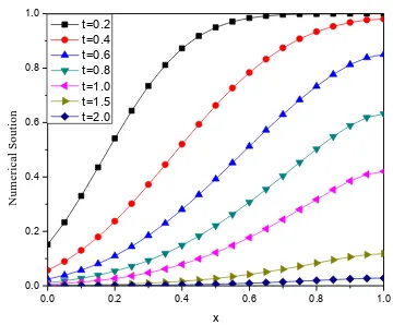
different times up to t=2. Figure 1 shows the behavior of the numerical solution at P=5.0 for different values of t. It is observed that at smaller value of t=0.2 the behavior of the numerical solution is almost flat and with the increase of
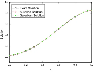
it shows exponential behavior. Figure 2 shows the variation of
the exact solution at P=5.0 for different values of t. Figures
3-4 shows the behavior of numerical solutions and the exact
solution at t=0.6 for different values of P. It is observed that
numerical solutions (Galerkin and B-spline) and the exact
solution are approximately same, which shows the validation
of purposed method.
Problem 2:
In this problem, we have considered the problem (16) with the
following initial and Dirichlet’s boundary conditions as
follows
1
C
, att
0
, for allx
0
C
atx
0
, and
0
x
C
, at
x
1
, for all0
t
, (17)The problem is again solved with the proposed
methods. The results of the problem are shown in the Figures
5-8. Figure 5 shows the behavior of numerical solution at P=5
at different values of t. It is observed as the value of t increases the solution becomes exponential. Figure 6 shows
the behavior of exact solution at P=5 at different values of t.
Figures 7-8 show the behavior of numerical solutions and
exact solution at t= 0.6 at different values of P. It is again observed that numerical solutions (Galerkin and B-spline) and
the exact solution for example 2 are approximately same,
which shows the validation of purposed method.
5. CONCLUSION
In this article, finite element is applied to two point boundary
value problem using quadratic B-spline basis functions. As
test problem, two different problems are considered. Firstly,
the problem is solved with B-spline finite element method
then the results are compared with both simple Galerkin finite
element method and the exact solution of the problem. It is
found that the proposed scheme has good accuracy.
0.0 0.2 0.4 0.6 0.8 1.0 0.0
0.2 0.4 0.6 0.8 1.0
N
u
m
e
ri
c
a
l
S
o
u
ti
o
n
x t=0.2
[image:4.595.334.514.86.235.2]t=0.4 t=0.6 t=0.8 t=1.0 t=1.5 t=2.0
Figure 1: The physical behavior of numerical solution of
Example 1 for
P
5
.
0
0.0 0.2 0.4 0.6 0.8 1.0 0.0
0.2 0.4 0.6 0.8 1.0
E
x
a
c
t
S
o
lu
ti
o
n
x t=0.2
[image:4.595.324.527.310.689.2]t=0.4 t=0.6 t=0.8 t=1.0 t=1.5 t=2.0
Figure 2: The physical behavior of exact solution of
Example 1 for
P
5
Figure 3: Comparison of all the solutions of Example 1 for P=5 and t= 0.6.
0.0 0.2 0.4 0.6 0.8 1.0 0.0
0.1 0.2 0.3 0.4 0.5 0.6 0.7
Sol
u
ti
o
n
x
[image:4.595.325.526.491.680.2]Figure 4: Comparison of all the solutions of Example 1 for P=10 and t= 0.6.
0.0 0.2 0.4 0.6 0.8 1.0 0.0
0.2 0.4 0.6 0.8 1.0
N
u
m
e
ri
c
a
l
so
lu
to
n
s
x t=0.2
[image:5.595.67.265.84.237.2]t=0.4 t=0.6 t=0.8 t=1.0 t=1.5 t=2.0
Figure 5: The physical behavior of numerical solution of
Example 2 for
P
5
0.0 0.2 0.4 0.6 0.8 1.0 0.0
0.2 0.4 0.6 0.8 1.0
E
x
a
c
t
S
o
lu
ti
o
n
x t=0.2
t=0.4 t=0.6 t=0.8 t=1.0 t=1.5 t=2.0
Figure 6: The physical behavior of exact solution of
Example 2 for
P
5
[image:5.595.328.526.291.438.2]Figure 7: Comparison of all the solutions of Example 2 for P=5 and t= 0.6.
Figure 8: Comparison of all the solutions of Example 2 for P=10 and t= 0.6
6. REFERENCES
[1] Jang B (2008). Two-point boundary value problems by the extended Adomian decomposition method. Journal of Computational and Applied Mathematics 219(1), pp. 253-262.
[2] Brenner H (1962). The diffusion model of longitudinal mixing in beds of finite length. Numerical values. Chemical Engineering Science 17(4), pp. 229-243. [3] Sharma D, Jiwari R and Kumar S (2011). Galerkin-finite
element methods for numerical solution of advection- diffusion equation. International Journal of Pure and Applied Mathematics 70(3), pp. 389-399.
[4] Noye BJ (1990). Numerical solution of partial differential equations, Lecture Notes.
[5] Dogan A (2004). A Galerkin finite element approach of Burgers’ equation. Applied Mathematics and Computation 157(2), pp. 331-346.
[6] Sengupta TK, Talla SB and Pradhan SC (2005). Galerkin finite element methods for wave problems. Sadhana 30(5), pp. 611-623.
[7] Kaneko H, Bey KS and Hou GJW (2006). Discontinuous Galerkin finite element method for parabolic problems. 0.0 0.2 0.4 0.6 0.8 1.0
0.0 0.2 0.4 0.6 0.8 1.0
Exact Solution B-Spline Solution Galerikan Solution
Sol
u
ti
o
n
x
0.0 0.2 0.4 0.6 0.8 1.0 0.0
0.2 0.4 0.6 0.8
1.0 Exact Solution
B-Spline Solution Galerikan Solution
Sol
u
ti
o
n
x
0.0 0.2 0.4 0.6 0.8 1.0 0.0
0.2 0.4 0.6
0.8 Exact Solution B-Spline Solution Galerikan Solution
Sol
u
ti
o
n
[image:5.595.74.253.297.443.2]Applied Mathematics and Computation 182(1), pp. 388-402.
[8] EI-Gebeily MA, Furati KM and O’Regan D (2009). The finite element-Galerkin method for singular self-adjoint differential equations. Journal of Computational and Applied Mathematics 223(2), pp. 735-752.
[9] Jangveladze T, Kiguradze Z and Neta B (2011). Galerkin finite element method for one nonlinear integro-differential model. Applied Mathematics and Computation 217(16), pp. 6883-6892.
[10] Padmaja P, Chakravarthy PP and Reddy YN (2012). A nonstandard explicit method for solving singularly perturbed two point boundary value problems via method of reduction of order. International Journal of Applied Mathematics and Mechanics 8(2), pp. 62-76.
[11] Kumar R, Kumar S and Miglani A (2010). Boundary value problem in fluid saturated incompressible porous medium due to inclined load. International Journal of Applied Mathematics and Mechanics 6(13), pp. 11-27. [12] Shabani MO and Mazahery A (2011). Application of
finite element method for simulation of mechanical properties in A356 alloy. International Journal of Applied Mathematics and Mechanics 7 (5), pp. 89-97. [13] Pathak AK and Doctor HD (2011). Comparison of
collocation method – spline, finite difference and finite element method for solving two dimensional parabolic partial differential equation. International Journal of Applied Mathematics and Mechanics 7(18), pp. 56-68.
[14] Mittal RC and Jiwari R (2009). Numerical study of burger-huxley equation by differential quadrature method. International Journal of Applied Mathematics and Mechanics 5(8), pp. 1-9.
[15] Chun C and Sakthivel R (2010). Homotopy perturbation
technique for solving two-point boundary value problems- comparison with other methods. Computer Physics Communications. 181 (6), pp. 1021-1024.
[16] Keller H B (1968). Numerical methods for Two-point
boundary value problems. Blaisdell Mass.
[17] Sharma D, Jiwari R and Kumar S (2012). Numerical
solution of two-point boundary value problems using Galerkin-Finite element method. International Journal of Non-linear Science. 13(2), pp. 204-210.
[18] Fox L (1957). The numerical solution of Two-point
boundary value problems in ordinary differential equations. Oxford University Press.
[19] Bellman R E and Kalaba R E (1965). Quasilinearization
and nonlinear boundary value problems. Rand Corp.
[20] Sharma D, Jiwari R and Kumar S (2012). A comparative study of Model matrix and Finite element methods for two-point boundary value problems. International Journal of Applied Mathematics and Mechanics 8 (13), pp. 29-45.