Munich Personal RePEc Archive
Endogenous Information Acquisition on
Opponents’ Valuations in
Multidimensional First Price Auctions
Tian, Guoqiang and Xiao, Mingjun
September 2007
Online at
https://mpra.ub.uni-muenchen.de/41214/
Endogenous Information Acquisition on Opponents’ Valuations
in Multidimensional First Price Auctions
∗Guoqiang Tian
Department of Economics
Texas A&M University
College Station, Texas, 77843
U.S.A
Mingjun Xiao
School of Economics
Shanghai University of Finance and Economics
Shanghai, 200433
China
January 9, 2009/Revised January, 2010
Abstract
This paper investigates bidder’s covert behavior of endogenous information acquisition
on her opponents’ valuations in first price auction model with independent private values.
Such an information acquisition setting leads to bidimensional type space and bidimensional
strategy space. We consider two different specifications of the environments: the ex ante
information acquisition setting and theinterim information acquisition setting. In equilibria
the expected payoffs of the bidder under these specifications could exceed the counterpart
payoffs of the corresponding standard sealed-bid auctions without information acquisition as
long as the cost is small, but the auctioneer has lower payoffs in these models than those
of the standard ones. Moreover, the incurred information cost becomes the deadweight loss,
resulting in inefficient outcomes.
Key words: First-price sealed-bid auctions, endogenous information acquisition,
oppo-nents’ valuation, profitability.
JEL Classification: C70; D44; D82.
1
Introduction
The information acquisition problem in auctions occurs when a bidder does not have a clear
idea about her exact willingness to pay for the underlying auctioned object, which can happen
in both common value auctions and private value auctions. Much work has been done on this
problem. This paper considers another type of information acquisition problem in which the
bidder knows her valuation of the auctioned object and also tries to learn the other bidders’
valuations. Thus each bidder has a bidimensional type that consists of her own valuation (the
valuation type) and the signal about her opponent’s valuation (information type).
In realistic economic activities, like auctions or procurement, and other similar situations,
bidders can have information about their own estimations of the auctioned object or project, and
also information about their opponents’ evaluations of the underlying object besides their
com-mon prior. The latter information may come from bidders’ strategic actions or from some other
parties, which helps update bidders’ beliefs on opponents. In other words, this is an environment
where bidders have multidimensional information, or multidimensional types in game theory
ter-minology. For example, in China, many middle-size and small-size state-owned enterprises have
been privatized by way of procurement in the past several years. There are usually two or three
potential buyers. The interactions between these buyers are rather involved and they may know
part of their opponents’ inside information. Another example is the NBA draft. The recruiting
competition can be compared to an auction over the top-ranked candidates by assuming that
the preferences of candidates only rely on monetary benefit. It has been observed during the
period that clubs take measures to hide their own beliefs about candidates’ values, and employ
“detectives” to investigate the confidential information on other clubs’ prices for recruiting their
desired candidate(s). We can see that a club could have multidimensional information, its own
evaluation and possibly other clubs’ evaluations of candidates in this competitive environment.
This paper tries to capture such a multidimensional information structure by way of
infor-mation acquisition1 on opponents. For independent private values, the bidder’s own valuation
does not tell her any information about other bidders’ valuations. This means the bidder
can-not update her belief based on her own valuation signal. A natural question, then, is whether
the bidder has incentives to acquire information about her opponents’ valuations. Though it is
somewhat difficult to find an example in the context of independent private value such that it
is fully consistent with this kind of information acquisition behavior, our paper makes the first
1
attempt to model bidders’ bidimensional types and bidimensional strategies in a simple setting.
The auction format we mainly focus on is the first price sealed-bid auction (abbreviated
as FPA), since this sealed-bid auction has been widely used in practice, such as in auctioning
mineral rights in government-owned land, the sales of artwork and real estate as well as
procure-ment. Examples include the U.S. offshore oil and gas lease auctions, the UK Treasury securities
auctions which are the multiunit equivalent of the first-price auction (every winner pays her own
bid).2 As Klemperer (2003, pp.2) has claimed, sealed-bid designs frequently (but not always)
both attract a larger number of serious bidders and are better at deterrence of collusion than
as-cending designs, see also Klemperer (1998, 2000, 2002). Maskin and Riley (1984) show that first
price sealed-bid auction is the most profitable one amongst the standard auctions when bidders
are risk-averse. When considering bidders have outside options, Kirchkamp et al. (2008) show
that bidders in first-price auctions have more overbidding with outside options than without,
and first-price auctions yield more revenue than second-price auctions do. As for second-price
sealed-bid auctions (SPA) or Vickrey Auctions, it might be trivial to consider such a type of
information acquisition on opponents’ valuations because opponents’ signals do not play any role
in the formulation of strategies in SPA. All these reasons lead us to consider first price auctions.
In our paper, the bidder can covertly incur a cost to achieve a noisy signal conveying
infor-mation about her opponents’ valuations. We assume neither the bidder’s inforinfor-mation acquisition
choice nor the signal received by the bidder can be observed by other bidders. For simplicity,
the accuracy of the signal and the cost of the signal are exogenously determined. In our
pri-vate value auction model, we analyze only the two-bidder case, where each bidder’s valuation
of the auctioned object is independently drawn from an identical distribution that has only two
possible values.
We consider two different specifications of the environments: theex ante information acquisi-tion setting where bidders invest in opponents’ valuaacquisi-tions before observing their own valuaacquisi-tions
and the interim information acquisition setting where bidders invest in opponents’ valuations after observing their own valuations. This is because both the interim and ex-ante information
acquisitions are equally interesting in daily economic activities. In some case one can obtain
information about one’s opponents prior to or when evaluating her own strength exactly in the
competition. For example, a firm needs to know about the incumbents of the market when it
considers entering that industry. In some case one may intentionally get to know his or her
com-petitors, namely, an incumbent would like to expect other firms’ reactions when it introduces
a new round of competition since the rivals’ strategies are of particular importance. In other
2
cases, one may know partial information on opponents as a byproduct with one’s own value and
then decide whether to invest in more.
Most studies of information acquisition in auctions focus on how to improve the estimate
of true valuation, since the bidder does not know her valuation when the auction begins, i.e.,
Matthews (1984) and Larson (2006) in the context of common values, Persico (2000) with
affil-iated values, Shi and Valimaki (2007) with interdependent values, Rezende (2005), Compte and
Jehiel (2007), Shi (2007) in private value settings. All these papers share the same characteristic
that bidders do not know their exact valuations at the beginning of the auction. Tan (1992)
and Arozamena and Cantillon (2004) investigate the incentives for investment before auctions,
and Hernando-Veciana (2006) considers the incentives of a bidder to acquire information in an
auction when her information acquisition decision is observed by the other bidders before they
bid.3
Our models have some similarities with that of Persico (2000), in which the bidder’s strategy
is bidimensional (consisting of the cost to induce more accurate signal and the bidding rule).
In our paper, the bidder’s strategy is also two-dimensional, namely, the bidder has freedom to
choose the probability to incur a fixed cost for receipt of a signal with certain accuracy and
specifies her bidding rules accordingly. However, the basic structures of the two papers are quite
different. Our paper also shares some common characteristics with Fang and Morris (2006).
First, both papers study the independent private value auction model where the bidder knows
exactly what her valuation is at the beginning of the auction. In addition, the costly information
acquisition behavior refers to collecting information about opponents’ valuations.
However, these two models have the following distinctions. First, in Fang and Morris’ model,
the behavior of acquiring information is exogenously given. Our paper aims to solve this problem
by endogenizing the choice of information acquisition, since in many realistic economic activities
the choice of acquiring information is part of bidders’ strategies. Secondly, there is no social
welfare loss in Fang and Morris’ binary-valuation model since no information cost is taken into
consideration. As such, the outcome is efficient from the view of social planner, which may be
regarded as “first best” outcome. However, contrary to Fang and Morris’ benchmark case, in
our model, costly information acquisition that can be regarded as an information rent leads to
deadweight loss in total social surplus, and consequently, it results in inefficient outcome, which
may be regarded as “second best” outcome4. In other words, generally information acquisition
3
There is also a strand of papers studying information acquisition problem where the auctioneer has controlled the information resources, such as Bergemann and Pesendorfer (2002) and Ganuza (2004), Eso and Szentes (2007). Milgrom and Weber (1982) also investigate the seller’s information disclosure policy in affiliated setting.
4
involves efficiency loss and the first best outcome cannot be achieved. Thirdly, our strategy
space is two-dimensional, while in Fang and Morris’ model it is of single dimension.
The contribution of this paper is as follows. First, our model takes an initial step in
endo-genizing information acquisition on opponent’s valuations in independent private value models.
Second, in our endogenous model, both the type space and strategy space of bidders are
bidi-mensional,5 which differs from the current literature. Third, we find that costly information
acquisition leads to deadweight loss in social surplus, and therefore, the equilibrium outcome
is inefficient. This tells that the efficient outcome is generally not achievable with costly
in-formation acquisition, and the corresponding policy implication would be that the inin-formation
acquisition behavior should be prevented to maximize social welfare.
The remainder of this paper is organized as follows. Section 2 describes the basic setting of
the model. Section 3 discusses bidders’ behavior when bidders can make ex ante information
acquisition choices. Section 4 considers a more relaxed environment in which bidders make
their information acquisition choices at an interim stage. Section 5 discusses the comparative
statics and implications: efficiency, surplus, and revenue across FPA and SPA formats. Section
6 discusses some variants of the model. Section 7 concludes. All the proofs are relegated to the
appendix.
2
Preliminaries
There are two risk neutral bidders indexed by i∈ N = {1,2} who compete for an underlying object. The object is worth zero to the seller. Every bidder i∈ N has a valuation vi ∈ V =
{Vl, Vh} for the object, where 0 < Vl < Vh. The valuations vi are private and independently drawn from identical distribution. The prior distribution of bidder i’s valuation vi is given by P r{vi = Vl} = pl (0 < pl < 1), and P r{vi = Vh} = ph = 1− pl for i ∈ N. Then
v = (v1, v2) ∈ V × V is a profile of possible valuations. The auction format is the first price
sealed-bid auction. The reservation price of the seller is normalized to zero.
Each bidder i can incur an exogenous costc(c ≧ 0) to get a noisy signalsi which induces information about her opponent’s private valuation. If the bidder does not want to collect
information about her opponent’s valuation, she does not incur any cost and cannot receive any
signal. Let ai ∈ {1,0} denote bidder i’s choice of acquiring information, where ai = 1 means
5
acquiring information andai = 0 means not.
To clearly describe the information structure, we assume neither the bidder’s information
acquisition choice nor the signal received by the bidder can be observed by her opponent.
The signal si received by bidder i is drawn from the support S = {L, H} if she acquires information. For convenience, we denote s0 as receiving no signal, and let ¯S = {L, H, s0}.
Given bidderj’s valuation and bidderi’s IA choice, the probability of the transmitted signalsi taking on each possible value is characterized by
Pr{si =L|vj =Vl, ai = 1}= Pr{si =H|vj =Vh, ai= 1}=q, Pr{si =s0|vj =Vl, ai= 0}= Pr{si =s0|vj =Vh, ai = 0}= 1;
(1)
for i6=j, i, j ∈ N; note that Pr{si = L|vj = Vl, ai = 1}+ Pr{si = H|vj = Vl, ai = 1} = 1 and Pr{si = H|vj = Vh, ai = 1}+ Pr{si = L|vj = Vh, ai = 1} = 1. Since all the signals are characterized by one parameterq, we callqthe accuracy of the signal. Without loss of generality, we assume 0.5< q ≦1. Bidder j updates her belief about i’s information type si according to the signal distribution specified by equation (1).
The auction game we will analyze is a Bayesian game of incomplete information. The
type space of each bidder is T ≡{Vl, Vh}×{L, H, s0}. One representative type of bidder i is
ti = (vi, si) ∈ T. We call vi the valuation type, and si the information type. Given bidder i’s signal si, bidder i updates her belief on her opponent’s valuation type according to the Bayes’ rule as follows. For si ∈ {L, H},i6=j, i, j ∈ N,
Pr{vj =Vl|si =L}=
plq
plq+ph(1−q)
,
Pr{vj =Vl|si =H}=
pl(1−q)
pl(1−q) +phq
,
Pr{vj =Vl|si =s0}=pl;
(2)
and the conditional probability is also a probability distribution, i.e., Pr{vj = Vh|si} = 1− Pr{vj =Vl|si} forsi∈S¯.
The primitives of the model are a tuple of five independent parameters as follows,
E =
½
< Vl, Vh, pl, q, c >: Vh > Vl>0, pl∈(0,1), q∈(0.5,1], c≧0
¾
.
3
Ex Ante Endogenous Information Acquisition
3.1 The Model
In this section we consider an auction economy in which bidders can acquire information on their
opponents’ valuations ex ante. That is, the bidder can decide whether to collect information before knowing her own valuation.
The procedures of this auction game are as follows:
• Stage 1. Bidders simultaneously decide whether to incur a costcto collect information on her opponent’s valuation, and this decision is not observed by her opponent.
• Stage 2. Nature draws a valuation for each bidder and tells the bidder only what her own valuation is. Every bidder receives a signal si revealing her opponent’s valuation if she incurs a costcin Stage 1. Otherwise, she receives no signal. Bidders’ signal is unobservable for her opponent.
• Stage 3. Bidders submit their bids simultaneously based on their own valuations, and possibly their updated belief from the signal according to (2).
• Stage 4. The bidder whose bid is the highest receives the object and pays what she bids.6
In this ex ante IA auction game, bidder has bidimensional type (valuation type and infor-mation type) and bidimensional strategy (acquiring inforinfor-mation choice and bidding rule). To
analyze this auction economy, we first define a set of notations.
For interested primitive values, bidders may randomize IA choice and bid submitted. Let
Fa({0,1}) denote the collection of probability distributions defined on the set {0,1}, and let
Fb([0, Vh]) denote the collection of probability distributions defined on the interval [0, Vh]. We define the bidder’s (mixed) strategy as follows. The (mixed) information acquisition choice
of bidder i is one element of Fa({1,0}), which can be simply characterized by one number
πiE = Pr{ai = 1} where 1 > πiE > 0 (note that 1−πiE = Pr{ai = 0}). A bidding rule7 is a mapping B ∋ b: T −→ Fb([0, Vh]). The strategy space of bidder iis then characterized by
6
When there is a tie, we choose the fair tie-breaking rule forq ∈ (0.5,1) and Vickrey tie-breaking rule for
q= 1. The fair tie-breaking rule says in the tie each bidder wins the object with equal probability and pays what she bids conditional on winning. The Vickrey tie-breaking rule is as follows: in the tie both bidders are asked to report a number, either 0 orǫ∗ where ǫ∗ is a sufficiently small positive number. If only one bidder reportsǫ∗, then this bidder gets the object and pays her bid; else the bidders get the object with equal probability and the bidder having the object pays her bid plus her reported number. Actually it does not matter which tie-breaking rule is used forq <1, we just choose the fair tie-breaking rule to explicitly and conveniently specify the strategic form of the auction economy. Forq= 1, however, the fair tie-breaking rule does not promise an equilibrium in our auction game and the Vickrey rule will reinstall the equilibrium.
7
AE
i =Fa({1,0})× B, and a typical element of AEi would be AEi = [πiE,(bi(t))t∈T]. Note that
bi(t) represents a random variable (or equivalently a distribution) with potential support [0, Vh], not a single bid. ThenAE =AE
1 × AE2 denotes the strategy space of the auction game.
Given a strategy profile (AE
1, AE2)∈ AE, there would be anex ante joint distribution of the
random vector (a1, v1, b1;a2, v2, b2), Γ(a1, v1, b1;a2, v2, b2|AE1, A2E) induced by (AE1, AE2), herebi refers to the bid that bidder i submits. The ex post payoff gE ≡ (gE
1, g2E) : {1,0}2 × V2 ×
[0, Vh]2 −→R2 simply takes the form as follows according to the first price auction rule
giE(a1, v1, b1;a2, v2, b2) = (vi−bi)·
·
1{bi> bj}+ 1
21{bi=bj}
¸
−aic, i6=j, i= 1,2, (3)
where 1{·} is the indicator function. Hence, the ex ante expected payoff GE ≡ (GE1, GE2) :
AE −→R2 is given by
GEi (AE1, AE2) =EΓ(·|AE
1,A
E
2) ·
giE(a1, v1, b1;a2, v2, b2)
¸
, i= 1,2, (4)
where the expectation of gEi is taken with respect to the joint distribution of random vector (a1, v1, b1;a2, v2, b2) induced by (AE
1, AE2).
A tuple <AE, GE >with primitive e∈E is then called an ex ante IA auction game.
3.2 Equilibrium
We first have the following lemma that tells type-Vlbidder bids her valuationVl for sure in any equilibrium.
Lemma 1 In any equilibrium of the ex ante IA auction game <AE, GE >, type-(V
l, s) bidders
bid Vl in pure strategy fors∈ {H, L, s0}.
With this lemma in hand, we establish that the equilibrium for this FPA auction game
<AE, GE > is unique and symmetric. The characterization of the equilibrium is summarized in the following proposition.
Proposition 1 The ex ante IA auction game <AE, GE > with primitive e∈ E has a unique
equilibrium. More specifically:
(i). When the informative cost is small, i.e. c < plp2h(Vh − Vl)(2q −1), then the unique
equilibrium of the FPA is symmetric and can be described as follows. For i= 1,2
1. With probabilityπE, the bidder collects information about her opponent’s private
2. bi(Vl, s) =Vl for s∈ {s0, L, H}.
3. When q = 1, type-(Vh, L) bidder submits bi(Vh, L) =Vl for sure; when q < 1, type-(Vh, L) bidder mixes over (Vl, δ1] according to the cumulative distribution function
(c.d.f ) Jl(·) specified by
Jl(b) = plq
πEph(1−q)2 ·
b−Vl
Vh−b
, b∈(Vl, δ1]. (5)
4. Type-(Vh, s0) bidder mixes over [δ1, δ2]according to the c.d.f. Js0(·) specified by
Js0
(b) = pl+πE(1−q)ph
ph(1−πE) ·
b−δ1
Vh−b
, b∈[δ1, δ2]. (6)
5. Type-(Vh, H) bidder mixes over [δ2, δ3]according to the c.d.f. Jh(·) specified by
Jh(b) = pl(1−q) +phq(1−πEq)
πEphq2 ·
b−δ2 Vh−b
, b∈[δ2, δ3]. (7)
Here
δ1 =
plqVl+πEph(1−q)2Vh
plq+πEph(1−q)2
, (8)
δ2 =
ph(1−πE)Vh+ [pl+πE(1−q)ph]δ1
pl+ph(1−πEq)
, (9)
δ3 =
πEphq2Vh+ [pl(1−q) +phq(1−πEq)]δ2
pl(1−q) +phq
, (10)
and πE is determined by the following condition:
ph
©
plq(Vh−Vl) + [pl(1−q) +phq(1−πEq)](Vh−δ2)ª−c
=ph
£
pl+πE(1−q)ph
¤
(Vh−δ1).
(11)
(ii). Whenc ≧ plp2h(Vh−Vl)(2q−1), the unique equilibrium of the FPA is symmetric and can
be described as follows. For i= 1,2
1. πiE = 0. No bidder acquires information.
2. bi(Vl, s0) =Vl.
3. Type-(Vh, s0) bidder mixes over (Vl, γ] according to the c.d.f. J¯(·) specified by
¯
J(b) = pl
ph ·
b−Vl
Vh−b
where
γ =plVl+phVh. (13)
Remark 1 Provided that the informative cost is negligible, i.e.,c= 0, the information acquisi-tion probabilityπE reduces to 1, which is the same equilibrium outcome as that of the exogenous information acquisition (Proposition 1 in Fang and Morris, 2006).
Remark 2 Whenq = 1, the switch of tie-breaking rule does not change the variables of interest. For instance, the bidder’s expected surplus and seller’s revenue are continuous at q = 1. The reason is that the equilibria are exactly the same under fair breaking rule and Vickrey
tie-breaking rule for q <1.
Remark 3 For equilibrium strategies in part (i), if πE = 0, type-(Vh, L) and type-(Vh, H) bid-ders disappear, and the formulaJs0(
·) remains valid; ifπE = 1, type-(Vh, s0) bidder disappears,
and the formulasJl(·) andJh(·) remain valid.
The type of equilibrium depends on the value of the informative cost. There is information
acquisition only if the cost is small, i.e., c < plp2h(Vh −Vl)(2q−1). In equilibrium, the bidder with valuationVlalways bids her valuationVl. If bidders acquire information, the type-(Vh, L), type-(Vh, s0) and type-(Vh, H) bidders play mixed strategy in equilibrium, and type-(Vh, L)’s support is lower than type-(Vh, s0)’s support which is also lower than type-(Vh, H)’s. This is because type-(Vh, L) bidder perceives her opponent more likely to be type-Vlbidder, type-(Vh, H) bidder regards her opponent more likely as type-Vh bidder, and type-(Vh, s0) bidder still takes
her ex ante belief. Then their best responses would result in such a support ranking. When the
informative cost is large, namely,c≧ plp2h(Vh−Vl)(2q−1), no bidder acquires information and it degenerates to the standard FPA equilibrium with primitivee∈E.
The proof of the proposition is a little bit involved, but the basic idea is simple. It is always
true that if the bidder plays mixed strategy in submitting her bid, she should get exactly the same
expected surplus from any bid drawn from the corresponding support. This fact (indifference
condition implied by mixed strategy) can help pin down the c.d.f of the bid as well as the upper
or lower bound of the support. The same idea applies that the bidder should be indifferent
between acquiring information and not acquiring information if she plays mixed strategy in IA.
3.3 Demand for Information
Substituting δ1,δ2 and δ3 into (11) and rearranging terms yields the formula of the reverse
demand for information:
c=plph(Vh−Vl)·
plphq(2q−1)
plq+ph(1−q)2πE ·
(1−πE) (1−phqπE)
. (14)
Immediately, we have the following intuitive result as a corollary of Proposition 1.
Corollary 1 (Demand for Ex Ante Information) The probability of ex ante IA, πE, has the
following properties:
(i). For all given values q ∈ (0.5,1], πE is continuous in c for c ≧0, and strictly decreasing
in c for c∈[0, plph2(Vh−Vl)(2q−1)].
(ii). For all values c ≧0,πE is (weakly) increasing in accuracy q.
When the cost of the signal is small, i.e., c ≦ plp2h(Vh −Vl)(2q −1), the probability of acquiring information, πE, satisfies the usual law of demand. This is intuitive because a more costly signal provides less incentive for the bidder when the accuracy keeps fixed.
On the other hand, a more informative signal will help the bidder evaluate her opponent
more effectively, and hence is more attractive to the bidder, provided the cost does not change.
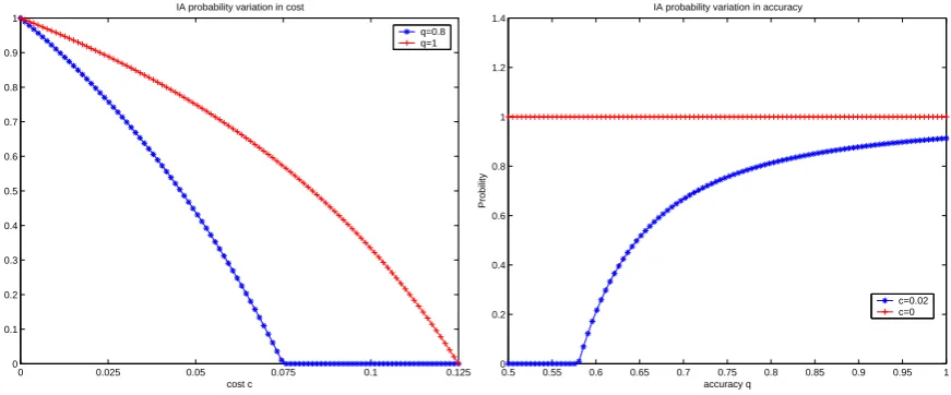
Quantitatively, Figure 1 presents the simulated results for the impacts of costcand accuracy
q on IA probability πE, respectively. It verifies the comparative results for πE. The primitive values are Vh = 2, Vl = 1 and pl = ph = 0.5, which are chosen for computing convenience. When considering the impact of the informative cost c, we choose two fixed values of accuracy,
q = 0.8 which is a representative of generic accuracy and q = 1 which represents the perfect accuracy. When considering the impact of the accuracyq, we fix the cost to be c = 0 (special costless case) andc= 0.02 (a representative of generic cost). These numeric values will be used continually in the following sections for consistency. The kink points in the figure correspond
to the critical values of cand q that satisfy the condition c=plph2(Vh−Vl)(2q−1). In the left sub-figure, the kink points are at critical valuec= 0.075 for q= 0.8 andc= 0.125 for q= 1. In the right sub-figure, the kink point is at the critical value q= 0.58 for c= 0.02.
In equilibrium, we see the type-Vl bidder ignores the signal received. Thus, one can expect that if we relax the endogenous information acquisition assumption, i.e., permitting collecting
information atinterimstage, the type-Vh’s demand for information can even be intensified. This is investigated in the next section. We will discuss the welfare analysis and comparative statics
0 0.025 0.05 0.075 0.1 0.125 0
0.1 0.2 0.3 0.4 0.5 0.6 0.7 0.8 0.9 1
IA probability variation in cost
cost c
Probability
q=0.8 q=1
0.5 0.55 0.6 0.65 0.7 0.75 0.8 0.85 0.9 0.95 1
0 0.2 0.4 0.6 0.8 1 1.2 1.4
IA probability variation in accuracy
accuracy q
Probility
[image:13.595.90.526.54.235.2]c=0.02 c=0
Figure 1: Cost and Accuracy’s Impacts on IA ProbabilityπE
Primitive: Vh = 2, Vl= 1, pl=ph= 0.5.
4
Interim Information Acquisition
In the previous section we consider the auction economy in which the bidder can freely choose
to collect information about her opponent’s valuation ex ante, but it is still very restrictive in the sense that the type-Vlbidder in the interim stage would definitely ignore the signal received. In other words, if the realized valuation is Vl, the bidder cannot benefit from the signal she receives because she cannot do better than bid her valuation Vl. In this section we consider the sealed-bid auction economy in which information acquisition choice is made after bidders’
valuations are realized, which will give the bidders more freedom to formalize their strategy in
the auction game.
4.1 The Model
The procedures of this auction game are as follows:
• Stage 1. Nature draws a valuation for each bidder and tells the bidder only what her own valuation is.
• Stage 2. Every bidder decides whether to incur a cost c to receive a signal si based on her valuation, and this decision as well as the signal received cannot be observed by her
opponent.
• Stage 3. Bidders submit their bids simultaneously based on their own valuations, and possibly the updated belief from the signal received according to (2).
In this interim IA auction game, bidder i’s strategy is a bidimensional mapping (ci,bi), such that C ∋ ci : {Vl, Vh} −→ Fa({0,1}) represents the IA choice rule and B ∋ bi : T −→
Fb([0, V
h]) represents the bidding rule, where AIi =C × B is bidder i’s strategy space. Denote ((c1,b1),(c2,b2)) = (AI1, AI2)∈ AI1× AI2≡ AI as one strategy profile.8
Similar as the ex ante IA setting, given a strategy profile (AI1, AI2)∈ AI, there would be anex
ante joint distribution of the random vector (a1, v1, b1;a2, v2, b2), Γ(a1, v1, b1;a2, v2, b2|AI
1, AI2)
induced by (AI1, AI2), here (ai, vi, bi) refers to the realization profile of bidder i’s information acquisition choice, valuation and bid sumbitted. Theex post payoffgI ≡(g1I, g2I) :{1,0}2× V2×
[0, Vh]2 −→R2 takes the same form as gE in (3), i.e.,
giI(a1, v1, b1;a2, v2, b2) = (vi−bi)·
·
1{bi> bj}+ 1
21{bi =bj}
¸
−aic, i6=j, i= 1,2. (15)
Hence, theex ante expected payoff GI≡(GI1, GI2) :AI −→R2 is given by
GIi(AI1, AI2) =EΓ(·|AI
1,A
I
2) ·
gIi(a1, v1, b1;a2, v2, b2)
¸
, i= 1,2, (16)
A tuple <AI, GI >with primitive e∈E is then called an interim IA auction game.
4.2 Equilibrium
The argument of Lemma 1 in the appendix does not require the detailed structure of
informa-tion acquisiinforma-tion, and therefore, the result that type-Vl bidder bids Vl in pure strategy in any equilibrium remains valid in our interim IA setting. Then only the type-Vhbidder has incentives to receive costly informative signal. Similarly, the equilibrium of the interim IA auction game
<AI, GI>is unique, symmetric and can be summarized as follows.
Proposition 2 The interim IA auction game < AI, GI > with primitive e ∈E has a unique
equilibrium. More specifically:
(i). When the informative cost is small, i.e. 0 ≦ c < plph(Vh−Vl)(2q−1), then the unique
equilibrium of the FPA is symmetric and can be described as follows. For i= 1,2
1. πiIl = 0. The type-Vl bidder does not incur any cost to receive any signal.
2. πiIh =πI. The type-Vh bidder, with probability πI, chooses to incur a cost c to collect
information on her opponent’s private valuation; with probability1−πI she does not
incur any cost.
8
ci is effectively referred to two distributions on binary support {1,0}. Hence, ci can be represented as
((πliI,1−π l iI),(π
h iI,1−π
h
iI)) whereπ l
iI = Pr{ai = 1|vi =Vl}denotes the IA probability of the type-Vl bidderi
andπh
3. bi(Vl, s0) =Vl.
4. When q = 1, type-(Vh, L) bidder submits bi(Vh, L) =Vl for sure; when q < 1, type-(Vh, L) bidder mixes over (Vl, β1] according to the c.d.f. Ql(·) specified by
Ql(b) = plq
πIph(1−q)2 ·
b−Vl
Vh−b
, b∈(Vl, β1]. (17)
5. Type-(Vh, s0) bidder mixes over [β1, β2]according to the c.d.f. Qs0(·) specified by
Qs0
(b) = pl+πI(1−q)ph
ph(1−πI) ·
b−β1
Vh−b
, b∈[β1, β2]. (18)
6. Type-(Vh, H) bidder mixes over [β2, β3]according to the c.d.f. Qh(·) specified by
Qh(b) = pl(1−q) +phq(1−πIq)
πIphq2 ·
b−β2
Vh−b
, b∈[β2, β3]. (19)
Here
β1=
plqVl+πIph(1−q)2Vh
plq+πIph(1−q)2
, (20)
β2=
ph(1−πI)Vh+ [pl+πI(1−q)ph]β1
pl+ph(1−πIq)
, (21)
β3=
πIphq2Vh+ [pl(1−q) +phq(1−πIq)]β2
pl(1−q) +phq
, (22)
and πI is determined by the following condition
plq(Vh−Vl) + [pl(1−q) +phq(1−πIq)](Vh−β2)−c
=[pl+πI(1−q)ph](Vh−β1).
(23)
(ii). Whenc ≧ plph(Vh−Vl)(2q−1), the unique equilibrium of the FPA is symmetric and can
be described as follows. For i= 1,2
1. πiIl =πhiI = 0. No bidder acquires information.
2. bi(Vl, s0) =Vl.
3. Type-(Vh, s0) bidder mixes over (Vl, γ] according to the c.d.f. J¯(·), where J¯(·) and γ
are given by (12) and (13), respectively.
Remark 4 As in the unique equilibrium of ex ante information acquisition, when the
Remark 5 For equilibrium strategies in part (i), if πE = 0, type-(Vh, L) and type-(Vh, H) bid-ders disappear, and the formulaQs0(·) remains valid; ifπ
E = 1, type-(Vh, s0) bidder disappears,
and the formulasQl(·) and Qh(·) remain valid.
In the unique equilibrium of interim information acquisition specified by Proposition 2,
type-Vl bidder has no incentive to acquire information and bids her valuationVl, type-Vh bidder plays a mixed strategy in information acquisition choice. The type-(Vh, L), type-(Vh, s0) and
type-(Vh, H) bidders randomly draw their bids in equilibrium, and type-(Vh, L)’s support is lower than type-(Vh, s0)’s, while the latter is also lower than type-(Vh, H)’s. This is similar to the bidding rule of ex ante information acquisition, so is the reason behind.
4.3 Demand for Interim Information
We callπI thedemand for interim information, since for any informative costc, the equilibrium is symmetric and unique.
The strategies in interim IA equilibrium share the same formulas as those in ex ante IA
equilibrium, except for the indifference condition that determines the probabilityπI. Obviously in interim IA setting, the typeVl bidder always gets zero surplus and has no incentive to acquire information, and the equation to pin down πI only concerns the type-Vh bidder. Therefore, the multiplier ph on both sides of (11) is eliminated, which yields (23). Again rearranging this equation yields the reverse demand for information in interim equilibrium, namely,
c=plph(Vh−Vl)·
plq(2q−1)
plq+ph(1−q)2πI ·
(1−πI) (1−phqπI)
. (24)
Parallel to the expression forπE, we have the property thatπI decreases as the cost goes up, the same as that in ex ante setting. And moreover, the interim demand for information,πI, is higher than the ex ante demandπE when facing the same cost in a proper range. These results are summarized in the following corollary.
Corollary 2 (Demand for Interim Information) The probability of interim IA, πI, has the
following properties:
(i). For all given values q ∈ (0.5,1], πI is continuous in informative cost c for c ≧ 0, and
strictly decreasing for c∈[0, plph(Vh−Vl)(2q−1)].
(ii). For all values c ≧0,πI is (weakly) increasing in accuracy q.
We have known qualitatively how bidders submit their bids in equilibrium. Now we give a
numeric example to illustrate their bidding rules and expected payoffs in equilibrium.
Example 1 Let Vh = 2, Vl = 1, q = 0.8, pl = ph = 0.5, c = 0.02. Then Table 1 gives
the probabilities of acquiring information at ex ante and interim stage, the endpoints of bidding supports and the corresponding expected payoffs (the formula of the expected payoff will be given in the next section). Figure 2 shows the mixing bid supports for this numeric example. Note that in standard first price auction without IA, the payoff of the bidder is 0.25, which is equal toplph(Vh−Vl).
Ex Ante Interim
πE 0.7170 πI 0.8572
δ1 1.0346 β1 1.0411
δ2 1.2261 β2 1.1453
δ3 1.5812 β3 1.6142
SE 0.2760 SI 0.2804
No IA
γ 1.5
[image:17.595.93.521.414.532.2]S0 0.25
Table 1: Example of IA and Bidding
γ
Interim IA
Ex Ante IA
Vl Vh
β1 β2 β3
Vl Vh
δ1 δ2 δ3
Figure 2: Bid Support
5
Discussion: Welfare Analysis and Comparative Statics
5.1 Ex Ante Information Acquisition
One central question that motivates our project is whether bidders benefit from acquiring
in-formation concerning opponent’s valuations. The answer is affirmative. Inin-formation acquisition
indeed improves the bidder’s surplus, albeit it cannot improve the allocative efficiency (the
since the information is costly and the expected social value of the object is fixed, the seller
nec-essarily raises less revenue. We will discuss how cost c and accuracyq impact bidder’s surplus and seller’s revenue as well as total social surplus in the following subsections.
5.1.1 Bidder’s Surplus
Bidder’s expected payoff in ex ante IA equilibrium has been given in the indifference condition
(11), either left or right hand side specifies the net surplus. By substituting δ1 into the right
hand side of (11), we have a simple formula for bidder’s expected payoff
SE = plq+phπEq(1−q)
plq+phπE(1−q)2 ·
plph(Vh−Vl), (25)
which is strictly increasing in the probability of acquiring information, πE when the signal is noisy but informative, i.e.,q ∈ (0.5,1). The standard FPA with the same primitive e will give the bidder surplus S0 =plph(Vh−Vl), which can be obtained by setting πE = 0 in (25). Note that the demand for information πE is decreasing in informative costcby Corollary 1, then we have the results summarized in the following proposition.
Proposition 3 Bidder’s net payoff in the ex ante IA auction game<AE, GE >with primitive
e, SE, has the following properties:
(i). SE exceeds the payoff in the standard FPA with primitivee, i.e.,SE≧S0 and the inequality
is strict forq ∈(0.5,1)and c < plp2h(Vh−Vl)(2q−1).
(ii). In the presence of noisy but informative signal, namely,q∈(0.5,1),SE is strictly decreas-ing in informative costc for c≦plp2h(Vh−Vl)(2q−1).
The proposition says the competition between bidders is not so fierce as that of the standard
FPA auctions. This is because by knowing more about the opponents’ valuations, type-(Vh, L) and type-(Vh, s0) bidders bid more conservatively, see the numerical Example 1. For instance,
the type-(Vh, L) bidder submits her bid very closely to Vl. The type-(Vh, H) bidder seems to bid more aggressively, i.e. in Example 1, the upper bound of her bid support δ3 = 1.5812 is
higher than γ = 1.5, the upper bound of type-Vh bidder’s support in standard FPA. However, on average, bidders with valuationVh bid less than they do in the standard FPA.
The accuracy q has a disparate impact on bidder’s payoff. An increment in accuracy has two effects. On one hand, a more accurate signal improves the bidder’s updated belief and the
bidder will bid more effectively if receiving the signal, which can increase the expected payoff.
On the other hand, a more informative signal reduces the bidder’s private information, and thus,
increases the competitiveness and leads bidder’s potential surplus to decrease. Theoretically, it
is not clear which effect dominates the other at all possible values of q. However, for extreme cases, we can see howq affects bidder’s surplus.
A very noisy signal provides bidders with no incentive to acquire information. It is easy to see
that the upper bound of the cost, beyond which no bidder will choose to acquire information,
plp2h(Vh −Vl)(2q −1) will be smaller than any given positive c if q stays sufficiently close to
1
2. Therefore, πE = 0 for q in some small neighborhood of 12. As the informativeness of the
signal improves,πE will be positive, hence the expected surplus of bidder goes aboveS0 in this
corresponding range ofq. On the other hand when the signal is completely accurate, i.e.,q= 1, bidder’s expected surplus falls back toS0by (25), which seems to be a little bit counterintuitive.
Note that whenq = 1, a type-(Vh, s) bidder cannot confront with a type-(Vh, L) opponent due to complete informativeness of the signal for all s ∈ {H, L, s0}. This reduces the probability
of winning against a relatively “weak” opponent, and therefore, leads to less expected surplus.
When q is somewhat informative but noisy, we do not know theoretically how bidder’s surplus changes asq increases. However, it seems that quantitatively the payoff is likely to increase first and then decrease as q goes up.
0 0.025 0.05 0.075 0.1 0.125
0.25 0.255 0.26 0.265 0.27 0.275 0.28 0.285 0.29
bidder surplus variation in cost
cost c
surplus
q=0.8 q=1
0.5 0.55 0.6 0.65 0.7 0.75 0.8 0.85 0.9 0.95 1
0.25 0.255 0.26 0.265 0.27 0.275 0.28 0.285 0.29
bidder surplus variation in accuracy
accuracy q
surplus
[image:19.595.87.534.453.639.2]c=0.02 c=0
Figure 3: Cost and Accuracy’s Impacts on Bidder’s Payoff
Primitive: Vh = 2, Vl= 1, pl=ph= 12.
Numerically, the comparative results can be seen in Figure 3, which confirms the comparative
regardless of the value ofq.
5.1.2 Total Surplus
In the unique equilibrium of ex ante information acquisition, the object is always optimally
allocated, so the total ex ante expected social welfare is equal to the expected value of max{v1, v2}
minus total expected informative cost. SinceE[max{v1, v2}] =pl2Vl+ (1−p2l)Vh and each bidder incurs expected informative costπEc, the total expected surplus then would be
T SE =p2lVl+ (1−p2l)Vh−2πEc. (26)
Note that if there is no information acquisition, the expected total social surplus would be
T S0 = p2lVl + (1−p2l)Vh by setting πE = 0 in (26). We can see the expected information cost 2πEc, which can be regarded as an information rent, becomes the deadweight loss. Hence, the ex ante IA equilibrium outcome is inefficient9 if bidders incur cost to acquire information,
which differs from the result in Fang and Morris’ binary value model that the exogenous IA
equilibrium outcome is always efficient due to zero-cost setting, which can be regarded as “first
best” outcome. Then the equilibrium outcome in our ex ante IA model may be regarded as
“second best” outcome, compared to the ideal case in Fang and Morris’ model.
The impacts of cost and accuracy on total surplus is then summarized in the following
proposition:
Proposition 4 The expected total social surplus in the ex ante IA auction game <AE, GE >
with primitivee, T SE, has the following properties:
(i). T SEis less than the social surplus in the standard FPA with the primitivee, i.e.,T SE≦T S
0
and the inequality is strict forq ∈(0.5,1)and 0< c < plp2h(Vh−Vl)(2q−1).
(ii). Suppose the accuracy q ∈ (0.5,1] is given, then T SE is decreasing in cost c for c ∈
[0, cE
T S(q)) and increasing in cost c for c∈[cET S(q), plp2h(Vh−Vl)(2q−1)], where cET S(q)∈ (0, plp2h(Vh−Vl)(2q−1)) is a constant dependent on q.
(iii). Suppose the costc∈(0, plp2h(Vh−Vl))is given, then T SE is weakly decreasing in accuracy
q∈(0.5,1].
We know that πE is decreasing when cost c goes up. It turns out that their product, the expected cost πEc first increases when cost is moderate and then decreases as cost becomes
9
large. Therefore, the total social surplus has a “U” shape response to cost. Provided the cost of
information acquisition is fixed, a more informative signal will increase the IA probability πE, hence the resulted social surplus decreases due to more expected cost. In other words, more
accurate signal actually hurts social benefit since the incurred information cost is deadweight
loss.
Figure 4 shows how social surplus reacts to the variation in cost c and to the variation in accuracy q, respectively, using the same primitive values as in previous numeric simulations. We can see no IA is the best outcome for the whole auction economy, and more accurate signal
makes the total welfare worse-off.
The above analysis implies that in realistic auction environment with information acquisition,
the efficient outcome is not generally achievable due to dissipative information cost. One policy
implication would be that information acquisition should be prevented to maximize the social
surplus. This can be done by means of raising the information cost or reducing the accuracy of
the signal or both. Or if possible, the central planner can directly control the IA choices to ease
social welfare loss.
However, when the cost is not a loss and is actually transferred to some party who provides
information, then information acquisition has no impact on social surplus. We will discuss it in
more detail in section 6.1.
0 0.025 0.05 0.075 0.1 0.125
1.6 1.625 1.65 1.675 1.7 1.725 1.75
total surplus variation in cost
cost c
TS
q=0.8 q=1
0.5 0.55 0.6 0.65 0.7 0.75 0.8 0.85 0.9 0.95 1
1.71 1.715 1.72 1.725 1.73 1.735 1.74 1.745 1.75 1.755
Total surplus variation in accuracy
accuracy q
TS
[image:21.595.80.535.411.595.2]c=0.02 c=0
Figure 4: Cost and Accuracy’s Impacts on Total Surplus
Primitive: Vh = 2, Vl= 1, pl=ph= 12.
5.1.3 Seller’s Revenue
The total social surplus contains two parts, the revenue of the seller and the surplus of the
bidders’ expected payoffs, namely,
χE = [p2lVl+ (1−p2l)Vh]−2πEc−2SE. (27)
Immediately by setting πE = 0 in (27), we know the revenue would be χ0 = [p2lVl+ (1−
p2l)Vh]−2S0 = (1−p2h)Vl+p2hVhin standard FPA. The equation (27) also tells us that the seller effectively bears the informative cost that is incurred by bidders. Note thatSE(q, πE) ≧ S0,
therefore, seller always gets revenue less thanχ0 in ex ante IA auction. Approximately, bidder’s
surplus and seller’s revenue change in opposite directions. To summarize, we have the following
comparative statics for seller’s revenue.
Proposition 5 Seller’s revenue in the ex ante IA auction game <AE, GE > with primitive e,
χE, has the following properties:
(i). χE is less than χ
0, seller’s revenue in standard FPA with primitive e, and the inequality
is strict forc < plp2h(Vh−Vl)(2q−1) andq ∈(0.5,1).
(ii). Suppose the signal is noisy but informative, namely, q ∈(0.5,1). Then there exists some constant cE(q) ∈ (0, plp2h(Vh −Vl)(2q −1)) dependent on q, such that χE is decreasing
in informative cost c for c ∈ [0, cE(q)) and increasing in cost c for c ∈ [cE(q), plp2h(Vh−
Vl)(2q−1)].
0 0.025 0.05 0.075 0.1 0.125
1.125 1.15 1.175 1.2 1.225 1.25
revenue variation in cost
cost c
revenue
q=0.8 q=1
0.5 0.55 0.6 0.65 0.7 0.75 0.8 0.85 0.9 0.95 1
1.15 1.16 1.17 1.18 1.19 1.2 1.21 1.22 1.23 1.24 1.25
revenue variation in accuracy
accuracy q
revenue
[image:22.595.84.533.372.616.2]c=0.02 c=0
Figure 5: Cost and Accuracy’s Impacts on Seller’s Revenue
Primitive: Vh = 2, Vl= 1, pl=ph= 12.
Obviously, seller’s revenue achieves its maximumχ0 only when bidders do not acquire
infor-mation (πE = 0, orc≧plph2(Vh−Vl)(2q−1)) or the signal is costless and completely informative (q = 1 and c = 0), according to the formula (27). Due to efficient allocation, bidders’ benefits would necessarily conflict with seller’s interest, which implies the seller would definitely prefer
no information acquisition. Then one policy implication would be that to raise more revenue,
the seller should prevent bidders from acquiring information, or induce either very noisy signal
or completely accurate signal whenever possible.
5.2 Surplus and Revenue in Interim IA Equilibrium
5.2.1 Bidder’s Surplus
Similar to ex ante IA equilibrium, bidder’s expected payoff in interim IA equilibrium has been
given in either side of the indifference condition (23). By substituting β1 into the right hand
side of (23), we have a simple formula for bidder’s expected payoff
SI = plq+phπIq(1−q)
plq+phπI(1−q)2 ·
plph(Vh−Vl). (28)
Hence we have the comparative results summarized in the following proposition.
Proposition 6 In the presence of noisy signal, i.e. q∈(0.5,1), and forc≦plph(Vh−Vl)(2q−1),
we have
(i). Bidder’s net payoffSI is decreasing in informative costc, and hence exceeds its counterpart
payoff, S0 from standard FPA without IA;
(ii). SI ≧ SE, and the inequality is strict for c∈(0, plph(Vh−Vl)(2q−1)) and q ∈(0.5,1),
provided the auctions <AE, GE > and <AI, GI > have the same primitivee∈E. This proposition is parallel to Proposition 3, and it says the impact of cost on bidder’s payoff
is similar to that of the ex ante IA case. When the signal is more costly, the type-Vh bidder would be less likely to acquire information, and bidder’s expected payoff goes down. Also the
accuracy of the signal has similar influence on bidder’s payoff as in ex ante case.
The information acquisition choice in interim stage becomes valuation-type-specific and turns
to be more efficient in terms of the utilization of the information. Hence bidders get higher ex
5.2.2 Total Surplus
In equilibrium of interim information acquisition, the object is optimally allocated, hence the
total expected social welfare equates to the total expected surplus minus total expected
infor-mative cost
T SI =p2lVl+ (1−pl2)Vh−2phπIc. (29)
Again similar to the ex ante IA case, the information cost 2phπIc turns to the deadweight loss, and the interim IA equilibrium outcome is not efficient, either.
Immediately, we have the following comparative results:
Proposition 7 The expected total social surplus in the interim IA auction game < AI, GI >
with primitivee, T SI, has the following properties:
(i). T SIis less than the social surplus in the standard FPA with the primitivee, i.e.,T SI≦T S0
and the inequality is strict forq ∈(0.5,1)and 0< c < plp2h(Vh−Vl)(2q−1).
(ii). Suppose the accuracyq ∈(0.5,1]is given, thenT SIis decreasing in costcforc∈[0, cIT S(q))
and increasing in costcfor c∈[cIT S(q), plp2h(Vh−Vl)(2q−1)], wherecIT S(q)∈(0, plp2h(Vh−
Vl)(2q−1)) is a constant dependent on q.
(iii). Suppose the cost c∈(0, plp2h(Vh−Vl))is given, then T SI is weakly decreasing in accuracy
q∈(0.5,1].
This proposition is parallel to Proposition 4, and the comparative results are similar in two
different IA settings. Unlike the bidder’s surplus, we cannot unambiguously rank the total
surpluses T SE and T SI. This is because the expected cost 2π
Ec in ex ante IA setting can be larger or smaller than the expected cost 2phπIc in interim IA setting.
5.2.3 Seller’s Revenue
Since total surplus includes seller’s revenue and bidders’ surpluses, then the revenue has the
following expression,
χI =p2lVl+ (1−p2l)Vh−2phπIc−2SI. (30)
Then we have the following results.
Proposition 8 Seller’s revenue in interim IA auction game <AI, GI > with primitive e, χI, has the following properties:
(i). χI is less thanχ0, seller’s revenue in standard FPA with primitive e, and the inequality is
(ii). Suppose the signal is noisy but informative, namely, q ∈(0.5,1). Then there exists some constant cI(q) ∈ (0, p
lph(Vh−Vl)(2q−1)) dependent on q, such that χI is decreasing in
informative costcforc∈[0, cI(q))and increasing in costcforc∈[cI(q), plph(Vh−Vl)(2q− 1)].
Quantitatively, bidder’s expected surplus and seller’s revenue have similar responses to the
cost and the accuracy of the signal as those in ex ante equilibrium, and the only difference
between ex ante and interim environments is the magnitude. We cannot generally tell whether
seller gets more revenue in the ex ante IA auction < AE, GE > or in the interim IA auction
<AI, GI>despite the unambiguous ranking for bidders’ surpluses in two different IA settings because it is not clear in which setting the expected cost is higher.
5.3 Comparison Across Auction Formats
It is obvious that the object is always efficiently allocated in our first price IA auction model since
bidders have binary values. As we have discussed at the very beginning, information acquisition
plays no role in formulating bidders’ strategies in second price auction (SPA) since each bidder
has weakly dominant strategy to bid truthfully, but it remains worth making comparisons across
FPA and SPA formats because the revenue equivalence still holds between these auctions without
any type of information acquisition.10
Consider SPA in our basic setting with primitive e ∈ E. The seller gets Vh if and only if
both bidders have valuesVh, which occurs with probability p2h, otherwise the seller receivesVl. Therefore in SPA, seller’s expected surplus, denoted byχSPA, would be
χSPA= (1−p2h)Vl+p2hVh. (31)
On the other hand, each bidder obtains positive surplus, i.e. (Vh−Vl) if and only if her own value is Vh and her opponent has value Vl, which occurs with probability plph. Then bidders’ expected surplus from SPA, denoted bySSPA, is
SSPA=plph(Vh−Vl). (32)
This yields the following results:
Proposition 9 Suppose 0< c < plp2h(Vh−Vl)(2q−1), q∈(0.5,1). Provided (FPA) IA games
<AE, GE >, <AI, GI>, and SPA are permitted in the basic setting e∈E, then we have
10
1. Bidder’s expected surplus from FPA is strictly higher than that from SPA, regardless of the stage at which the IA choice is made, i.e.,SE> SSPA
andSI > SSPA
.
2. Seller gets strictly less expected revenue from FPA than that from SPA, no matter at which stage bidder can acquire information, i.e.,χE< χSPA and χI< χSPA.
The first item could follow from Proposition 3 and Proposition 6, since the revenue
equiva-lence still holds with discrete values across standard FPA and SPA without information
acqui-sition, i.e.,SSP A=S0, and IA plays no role in formulating strategies in SPA.
The revenue ranking is unambiguously clear across FPA and SPA for our binary value
model.11 However, this ranking does not hold generally for endogenous IA. For example, when
valuation has continuous support, then it is possible that seller gets more revenue in FPA than
in SPA.
It is obvious that bidders have strong incentives to acquire information about their opponents’
valuations intentionally in FPA if it is permitted, but not in SPA. The other fact is that the
auctioneer is worse-off in FPA, if such an information acquisition occurs, which differs from the
result that revenue increases associated with traditional information acquisition. The natural
policy implication would be that the seller may need to deter bidders’ potential information
acquisition to maximize her revenue if bidders’ private values are independent.
6
Some Variants
6.1 Third Party Charges the Informative Cost
In our basic setting, we do not model where the informative signal comes from, i.e., who provides
the information. Therefore, in our welfare analysis, the informative cost becomes the deadweight
loss of total social surplus. Also, we leave it open for pricing the signal. It seems that the two
issues can be resolved by introducing the third party who actually collects information and sells
it to bidders.
Suppose there exists such a third party at ex ante stage(the case is similar at interim stage).
The party has the access to collect noisy information concerning bidders’ valuations without
in-curring any cost, and aims to maximize its total revenue from providing information. Therefore,
11
the third party has objective function
τE(c) = 2πEc. (33)
By Proposition 1, the possible informative cost charged by this party is the interval [0, plp2h(Vh−
Vl)(2q−1)]. If the accuracy of the transmitted signalq cannot be controlled by this party, then the optimal cost for this party would be cET S(q), which is the constant given in Proposition 4 item (ii). The interesting thing is that if the accuracy can be chosen by this party, then definitely
the party will choose optimal accuracyq∗ = 1 to maximize the expected cost 2πEcbecause πE is increasing inq by Corollary 1. However, bidders cannot benefit from this completely accurate signal since they can just get expected surplus SE = S
0. This optimal choice may favor the
seller to some extent, for bidders’ having less surplus means that seller may get more revenue
(increment in expected cost will reduce revenue at the same time).
One key point is that the expected total surplus now is always a constantT S=T S0 since the
expected cost – the deadweight loss – now turns to be the benefit of the third party. Therefore,
the IA auction game <AE, GE > becomes one mechanism that redistributes the total surplus amongst bidders, seller and the information provider. Moreover, part of seller’s revenue is
redistributed to bidders and the information provider compared to the standard FPA with the
same primitive, which can be easily seen from the formula (27).
6.2 Observable Information Acquisition
This paper considers covert information acquisition on opponent’s valuation, and it is crucial
to maintain the assumption that the choice of acquiring information is unobservable to the
opponent. It will result in two problems without this assumption. We consider the interim IA
setting. First, the signal structure is not inherently consistent. This is a model with binary
valuations, hence only the type-Vh bidder has incentive to acquire information. If this action is public information, then it is a perfect signal that tells bidder j vi = Vh when i acquires information. Also bidder j could be a type-Vh bidder who already acquires information and receives a signal sj, then sj is meaningless for the bidder, thus why should the bidder incur a cost to acquire information? Second, there could be no equilibrium in some subcases. Suppose
bidderihas valuation Vh and acquires information and bidder j does not, and this is common knowledge. In this case, no equilibrium bidding strategy exists with fair tie breaking rule.12
Hence observable information acquisition is undesirable for our modeling.
12
6.3 More Realizations
Besides the binary values, more points of valuation support could be added in. As Fang and
Morris (2006) have observed: it does not admit any equilibrium for exogenous information
acquisition with generic parameters even in binary valuation support model. Thus for more
points, the equilibrium analysis would also be problematic. As for continuous valuation support,
the formation of bidding rule with multiple arguments turns to be a rather involved problem,
which is the essential question with multidimension. This is an open question for future research.
6.4 Beyond Private Values
Admittedly, we specify an independent private value setting, which seems to be restrictive in
some sense. This endogenous IA specification can be extended to other non-private value
envi-ronment. For example, it turns out that in endogenous IA first-price auction with interdependent
discrete valuations, bidder can also get higher payoff than that of standard FPA without IA,
which is the environment we haven’t considered here but are working on.
7
Conclusion
This paper mainly investigates bidders’ covert information acquisition on opponents’ valuations
in first price sealed-bid auctions with independent private values, which leads to bidimensional
strategy space and bidimensional type space. We present two different specifications: ex ante
information acquisition and interim information acquisition. We find that: (i) bidder’s expected
payoff exceeds that of the counterpart standard FPA when informative cost is small and the
signal is informative and noisy; (ii) the auctioned object is always efficiently allocated due
to the settings of binary values; (iii) in all cases in which bidder acquires information with
positive probability, the auctioneer’s expected revenue is lower than that of the standard auction,
which contradicts the results in the current information acquisition literature; (iv) the incurred
informative cost becomes the deadweight loss in total social surplus and the equilibrium outcome
is inefficient. The natural implication of our analysis would be that seller needs to prevent bidders
from acquiring information to raise more revenue. Also from the social planner’s point of view,
information acquisition should be prevented to maximize social welfare. We also analyze how
the accuracy and the informative cost impact on bidders’ expected surplus, seller’s revenue and
total surplus. Some possible variations of the model are discussed at last.
Our paper takes the first step to explore the properties of endogenous information acquisition
have incentives to take this IA action. To see the robustness of the results, continuous support
necessitates exploration. It seems that the difficulty rests with the multidimensional bidding
rules. Moreover, the probability of acquiring information is probably a function of bidder’s
valuation. These are open questions for future exploration.
8
Appdendix
Proof of Lemma 1: Forti∈ {Vl} × {L, H, s0}, let type-ti bidderi’s bidding support be either [bti1, bti2] withbti1 ≦bti2 ≦Vlor (bti1, bti2] withbti1 < bti2 ≦Vl(the upper bound of the support interval may be open, but this is not important for the argument). Let t ∈ arg mint1∈{Vl}×{L,H,s0}b
t1
1
and t′∈arg mint2∈{Vl}×{L,H,s0}b
t2
1 .
We first show that type-t bidder 1 and type-t′ bidder 2 should bid in pure strategies. It is obvious that bt1 = bt1′ = b1 since bt1 and bt
′
1 are the possible smallest bids for bidders 1 and 2,
respectively. There are four possible cases that can be ruled out in equilibrium.
Case 1: type-tbidder 1 has support (b1, bt2] and type-t′ bidder 2 has support (b1, bt2′] where
b1 < bt
2 and b1 < bt
′
2. We can see that the bid b=
b1+min{bt2, b
t′
2}
2 will yield both type-t bidder 1
and type-t′ bidder 2 positive surplus. However, bids close to b1 will win with probability almost
zero, hence both bidder 1 and type-t′ bidder 2’s surpluses will approach zero by submitting a bid close tob1. This is a contradiction with the indifference condition given by mixed strategy,
so this pattern of the supports cannot be the case.
Case 2: type-t bidder 1 has support (b1, bt2] and type-t′ bidder 2 has support [b1, bt
′
2] where
b1 < bt2 and b1 < bt2′, or type-t bidder 1 has support [b1, bt2] and type-t′ bidder 2 has support
(b1, bt
′
2] where b1 < bt2 and b1 < bt
′
2. Since the two subcases are symmetric, consider the former
one. It is easy to see a bid b1 yields bidder 2 exactly zero surplus due to zero winning
prob-ability. However, a bid b = b1+min{bt2, b
t′
2}
2 yields bidder 2 strictly positive expected surplus, a
contradiction with the indifference condition. This pattern cannot be true either.
Case 3: type-t bidder 1 has support [b1, bt2] and type-t′ bidder 2 has support [b1, bt
′
2] where
eitherb1< bt2 andb1< b2t′, orb1 =bt2 andb1 < bt2′, orb1=b2t′ andb1 < bt2. Consider the subcase
where b1 < bt2. A bid
b1+bt2
2 will yield type-t bidder 1 positive surplus. Hence by indifference
condition, a bid b1 will give type-t bidder 1 positive surplus, which requires her opponent—
bidder 2 to submit a bid b1 with positive probability so that type-t bidder 1 can win against
bidder 2 with positive probability by submittingb1. However, then, if type-t bidder 1 submits
a bid slightly higher than b1, this bid will yield a jump in winning probability against bidder 2, hence a jump in expected surplus of type-tbidder 1. Again a contradiction with the requirement of mixed strategy. The subcase whereb1 < bt′
Case 4: type-t bidder 1 has support (b1, bt2] with b1 < bt2, type-t′ bidder 2 bids b1 with
probability 1; or type-t′ bidder 2 has support (b1, bt′
2] withb1 < bt
′
2, type-t bidder 1 bidsb1 with
probability 1. By symmetry, it suffices to consider the former subcase. It is obvious that type-t′
bidder 2’s strategy is not optimal. The bidb1 wins against none of bidder 1’s bids, hence yields bidder 2 zero surplus. By submitting a bid b1+bt2
2 , type-t′ bidder 2 gets strictly positive expected
surplus, which is a profitable deviation.
Since all those cases are excluded from equilibrium, we conclude that it must be true in
equilibrium thatb1 =bt2=bt
′
2. In other words, type-t bidder 1 and type-t′ bidder 2 bid in pure
strategies.
We then show that b1 =Vl. Suppose b1 < Vl, then either type-tbidder 1 or type-t′ bidder
2 can deviate by submitting a slightly higher bid b1 +ǫ with probability 1, which will be a
profitable deviation by choosingǫarbitrarily close to zero. A contradiction.
Note that b1 is the possible lowest bid for all types ti∈ {Vl} × {L, H, s0},i= 1,2 and those
bidders will never bid more than their valuationVl. The proof is complete.
Proof of Proposition 1: We take several steps to complete this argument. First we verify that
the provided strategies in the proposition actually constitute an equilibrium. Then we show that
there is no other symmetric equilibrium. Last we argue that there is no asymmetric equilibrium
either.
One point we would like to clarify before the formal proof is that in part (i) for q ∈(0,1), when q approaches 1 from below, the limit of type-(Vh, L)’s bid support (Vl, δ1] would be an
empty set due to limp→1δ1 = Vl. Hence type-(Vh, L) bidder’s best bidding strategy doesn’t exist given all other types’ bidding strategies. That’s why the tie-breaking rule needs to switch
at q = 1. Under Vickrey tie-breaking rule, type-(Vh, L)’s bid support could be closed interval [Vl, δ1](the limit of this interval is singleton{Vl}asp→1), and any other type bidder’s strategy does not change. The following argument considers the setting for q ∈ (0,1), and the same argument can go through for q = 1 (possibly with some slight modification) by replacing type-(Vh, L)’s bid support (Vl, δ1] with closed interval [Vl, δ1].
The argument follows several intermediate claims:
Claim 1. Given that the bidder’s opponent follows the provided strategy in the proposition, the bidder’s best response is the same strategy given in the proposition.
Note that by Lemma 1, it suffices to check the strategies of the bidders with valuation Vh. We just need to verify that the bidder gets exactly the same expected payoff if she submits any
bid drawn from the support of provided mixed strategy, and that the bidder cannot obtain more