The Estimation of the Error at Richardson’s Extrapolation and the Numerical Solution of Integral Equations of the Second Kind

(1)

How to cite this paper: Dobrovolsky, I.P. (2015)The Estimation of the Error at Richardson’s Extrapolation and the Numeri-cal Solution of Integral Equations of the Second Kind. Open Access Library Journal, 2: e2051.

http://dx.doi.org/10.4236/oalib.1102051

The Estimation of the Error at Richardson’s

Extrapolation and the Numerical Solution of

Integral Equations of the Second Kind

Igor Petrovich Dobrovolsky

Institute of Physics of the Earth, Russian Academy of Sciences, Moscow, Russia

Received 18 October 2015; accepted 3 November 2015; published 9 November 2015

This work is licensed under the Creative Commons Attribution International License (CC BY). http://creativecommons.org/licenses/by/4.0/

Abstract

The mode of definition of the error at polynomial Richardson’s extrapolation is described. Along with the table of extrapolations the new magnitudes reflecting expediency and efficiency of extrapolation are entered. On concrete examples it is shown that application of Richardson’s extrapolation to a solution of integral equations has appeared rather effective and gives a solution with a high exactitude. Application of formulas of interpolation leads to a solution in the analytical aspect.

Keywords

The Trapezoidal Rule, Continued Fraction, The Index of Richardson’s Extrapolation

Subject Areas: Geology, Geophysics

1. Introduction

Numerical methods of the approached solution are attractive by the universality. In numerical methods three problems are put: obtaining enough exact solutions, accuracy control and algorithmic simplicity of procedures. Richardson’s extrapolation solves these problems. The first work of this theme was [1]. Since then many works (for example [2]) are published and there is no necessity to do one more review. However, it is impossible to consider a theme exhausted. For example, in full enough handbook [3], there is no even a mention of application of Richardson’s extrapolation to a solution of integral equations.

The purpose of this paper is to construct procedure of an estimation of an error at Richardson’s extrapolation and to apply it to a numerical solution of integral equations of the second kind of Volterra and Fredholm.

2. About Polynomial Richardson’s Extrapolation

(2)

OALibJ | DOI:10.4236/oalib.1102051 2 November 2015 | Volume 2 | e2051

There are many problems from different sections of mathematics in which the difference between exact ϕ and approached ψ by solutions (an error of calculation of r) at sufficient smoothness of functions of a problem has expansion

( )

1

, ,

k

sn sk

n n

r x h ϕ x ψ x h v x h o h

=

= − =

∑

+ . (2.1)

Magnitude h is usually a grid step.

We shall designate the approached solution as

(

)

( )0

, _i _i

x h

ψ =ψ . (2.2)

( )0 i

ψ is called as extrapolation of the zero order.

Extrapolation of the 1-st order is obtained by elimination of the first term of expansion (2.1) by a linear com-bination of extrapolations of the zero order. Extrapolation of the j-st order is calculated on the recurrence for-mula

( ) (11) 1 ( 1)

1

j j

s s

j i i i i

i s s

i i

h h

ψ ψ

ψ +− + −

+ − =

− (2.3)

where usually is accepted h_i₊₁<h_i.

In the end a table of extrapolations is obtained

( ) ( ) ( ) ( )

( ) ( )

( )

0 1 2

1 1 1 1

0 1

2 2

0 2

3 2

1 1 0

m

ψ ψ ψ ψ

ψ ψ

−

   

. (2.4)

3. The Analysis of the Table of Extrapolations in Special Case

If magnitude h forms a geometrical progression

1 1

i i

h h

q−

= (3.1)

that (2.3) receives an aspect

( ) ( ) ( ) ( )

( )

1

1 1

1

s j j j

j i i

i s j

q

ψ ψ

ψ + + +

+ − =

− . (3.2)

In this case from (3.2) and (2.1) we have

( ) ( ) ( )1

1

j j sn i

i i jn

n j

r

ϕ ψ

a q− −

= +

= − =

∑

(3.3)

where lack of the top sign at the sum means that the remainder term is included in this sum. We will name as the index of extrapolation R_i( )j ratio

( ) ( )

( )

1

1 j j i

i j

i r R

r +

+

= . (3.4)

Extrapolation improves an exactitude ψ_i(j+1) in comparison with ψ_i( )₊j₁ when Ri(j 1) 1

− _<

. From (3.3) follows

( ) ( ) ( ) ( )1

1

j j j sn i

i i i jn n

n j

a B q

ψ

− −

+

= +

(3)

where B_n = −1 q−sn.

Because B_n ≈1 we have an obvious relation

( )j ( )j

i i

r ≈ −∆ . (3.6) By means of the Formula (3.5) table ∆( )_ij is created.

Obviously, at a diminution h there occurs such moment when terms in expansion (3.3) start to decrease mo-notonically. We name this mode regular. If extrapolation becomes on a regular mode, the first term should bring the basic contribution in expansion (3.5). Then the relation should be observed

( ) ( )

1

1 j

j i s j

i j

i q

δ +

+ ∆

= ≈

∆ . (3.7)

And on the contrary: if the relation (3.7) is observed, we have a regular mode. Magnitude δ_i( )j is almost constant in a table column. By means of the Formula (3.7) table δ_i( )j is created.

Let’s enter magnitude

( ) ( )

( )

( ) ( )

1 1

1

1 1

j j

j i i

i s j s j j

i

q q

δ

γ ₊ ₊

+ ∆

= − = −

∆ (3.8)

and we shall define its meaning. From (3.8), we have

( ) ( )

( )

(

( )

)

1 ₁

1

j

j i

i _{s j} _j

i

q γ

+ ₊

∆ ∆ =

− . (3.9)

Substituting (3.9) in (3.2) we receive

( ) ( ) ( )

( )

(

)

(

( )

)

1

1 1

j j

j i i

i _{s j} _j

i q

γ γ +

+ ∆

∆ =

− − . (3.10)

From (3.4), (3.6), (3.9) and (3.10) , we have

( ) ( )

( )

( ) ( )

1 1 1

1

1 1 1

j j s j

j i i j

i j j s j i

i i

r q

R

r q

γ

+ + +

+

+ +

∆

= ≈ =

∆ − . (3.11)

Therefore, γ_i( )j is estimation the index of extrapolation. By means of the Formula (3.8) table γ_i( )j is created.

By Formulas (3.6), (3.7), (3.11) and assumption γ_i( )j =γ_i(j−1) the error estimation is

( ) ( ) ( )

( )

1 1

1

j j

j i i

i s j

r

q γ − +

+ ∆ ≈ −

− . (3.12)

Starting from row (3.5) and definition (3.8), it is possible to establish that there is the expansion for γ_i( )j

( ) , 2 2

(

)

, 1 1

1 s

j j j

j si

i

j j j

a B q

q

a B

γ + + −

+ + −

= + (3.13)

where the first item has a basic meaning in a regular mode. Then from (3.13) we receive the relation

( )

1 j

s i

j i

q γ

γ₊ → at i→ ∞ (3.14)

(4)

4. The Numerical Solution of Integral Equation of Volterra

Let’s consider integral equation of Volterra of the second kind.

( )

( ) ( )

( )

0

, d

x

y x −

∫

K x t y t t= f x (4.1)

where f x

( )

= −

(

1 xe2x

)

cos1 e− 2xsin1 and K x t

( )

, = −1

(

x t−

)

e2x. This equation has an exact solution

( )

2

e cos ex x e sin ex x

y x = − . (4.2) We shall designate the approximate solution of the Equation (4.1) at the calculation of integrals on a trape-zoidal rule with extrapolation by y_i( )j .

Procedure of a solution of integral equation of Volterra of the second kind with application of the trapezoidal rule is known (for example [3]). At the calculation of integrals by the trapezoidal rule s = 2. At q = 2 each pre-vious set of points contains in the subsequent set and it enables application of extrapolation. Then (3.3) receives the form

( )

_{( )}

( )

_{( )}

( )1

_{( )}

1

4

j j n i

i i jn

n j

r x y x y x − − a x

= +

= − =

∑

(4.3)

and (3.2) receives the form

( ) ( ) ( ) ( )

( )

1

1 1

1

4

4 1

j j j

j i i

i j

y y

y

+

+ +

+ − =

− . (4.4)

It is sometimes more convenient to use “direct” formulas

( ) ( ) ( )

( ) ( ) ( ) ( )

( ) ( ) ( ) ( ) ( )

( ) ( ) ( ) ( ) ( ) ( )

0 0

1 1

0 0 0

2 2 1

0 0 0 0

3 3 2 1

0 0 0 0 0

4 4 3 2 1

4 3 64 20

45

4096 1344 84 2835

1048576 348160 22848 340 722925

i i

i

i i i

i

i i i i

i

i i i i i

i

y y

y

y y y

y

y y y y

y

y y y y y

y

+

+ +

+ + +

+ + + +

− =

− +

=

− + −

=

− + − +

=

(4.5)

which come out by sequential application of the Formula (4.4).

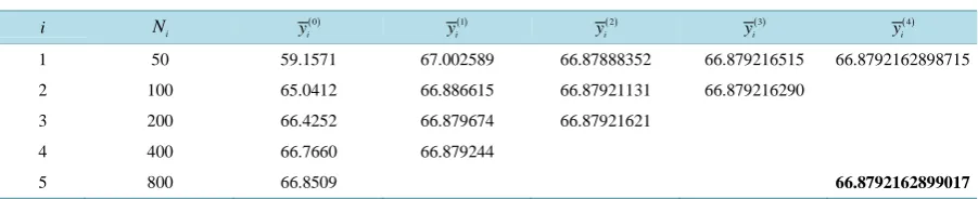
Let’s consider (4.1) on a piece x = 0 ÷ 2.5 with step h_i =2.5 N_i . Below tables of extrapolations and other magnitudes according to formulas of the previous section are reduced. Calculations were made with 15-th sig-nificant digits, but for convenience of reading in tables of number are approximated.

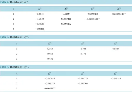
By means of the Formula (3.5) table ∆( )_ij is created. By means of the Formula (3.7) table δ_i( )j is created. By means of the Formula (3.8) table γ_i( )j is created.

[image:4.595.88.539.628.720.2]

The analysis of tables leads to the important conclusions. From Table 1 andTable 2 follows that y₁( )4 is the most exact value. It is visible from Table 3that the Formula (3.7) is satisfactorily satisfied. FromTable 4 follows,

Table 1.Table of extrapolation ( )j i

y in the point x = 2.5. The exact magnitude is shown by bold type.

i Ni

( )0 i

y ( )1

i

y ( )2

i

y ( )3

i

y ( )4

i

y

1 50 59.1571 67.002589 66.87888352 66.879216515 66.8792162898715

2 100 65.0412 66.886615 66.87921131 66.879216290

3 200 66.4252 66.879674 66.87921621

4 400 66.7660 66.879244

(5)

[image:5.595.87.538.85.398.2]

OALibJ | DOI:10.4236/oalib.1102051 5 November 2015 | Volume 2 | e2051 Table 2. The table of ( )j

i

∆ .

i ( )0

i

∆ ( )1

i

∆ ( )2

i

∆ ( )3

i

∆

1 −5.8841 0.1160 −0.0003278 6

0.22474 10× −

2 −1.3840 0.0069411 5

0.49005 10−

− ×

3 −0.34081 0.0004292

4 −0.08488

Table 3. The table of ( )j i

δ .

i ( )0

i

δ ( )1

i

δ ( )2

i

δ

1 4.2514 16.708 66.889

2 4.0611 16.171

3 4.0152

γ .

i ( )0

i

γ ( )1

i

γ ( )2

i

γ

1 −0.062845 −0.044273 −0.045144

2 −0.015275 −0.010703

3 −0.0037927

that γ_i( )j depends from j a little at everyone i. Now it is possible to make an estimation of the error of y_i( )4 at

x = 2.5. From (3.12) we have

( )4 ( ) ( )13 12 10

1 0.40 10

255

r ≈∆ γ = × − . (4.6) The true error is 0.30 10× −10.

We have received the precision solution in isolated points. It is interesting to find good interpolation function and to receive a solution in the analytical form. Let’s make uniform set from y₂( )3 with the step 0.1 (26 points). Interpolation by continuous fractions (the command Thiele Interpolation in the package Curve Fitting of the program Maple) was better than interpolation by cubic splines. Interpolation by continuous fractions we shall designate y( )₂3

( )

x and y₁( )4 serves as control value. These results are presented inTable 5.

The Equation (4.1) for area x≥a can be written down in the form.

( )

( ) ( )

( )

( ) ( )

0

, d , d

x a

a

y x − K x t y t t=_f x + K x t y t t_

 

∫

. (4.7)

The Equation (4.7) defines the solution at

x

>

a

if function y x

( )

is known at x≤a.

5. The Numerical Solution of Integral Equation of Fredholm

The equation is considered

( ) (

1

)

( 1)

_{( )}

1

0

1 ext d e

y x −

∫

+x − y t t= − (5.1)

which has the exact solution y=ex.

(6)

[image:6.595.171.512.425.603.2]

OALibJ | DOI:10.4236/oalib.1102051 6 November 2015 | Volume 2 | e2051 Table 5. Interpolation ( )4

1

y and exact solution

(

y x

( )

)

. At x = 2.488 interpolation has the largest error.

x = 2.488 x = 2.45 x = 2.35 x= 1.95

( )3_{( )} 2

y x 83.53814 117.853257 68.052110 –28.347394668

( )4 1

y 117.853249796849 68.05210963589 –28.3473946668611

( )

y x 83.53832 117.853249796861 68.05210963599 –28.3473946668607

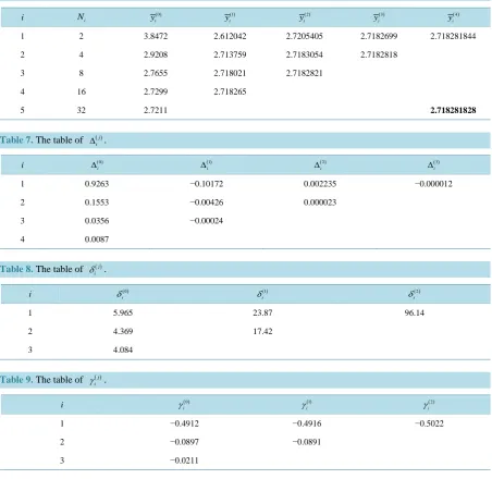
rule is also known (for example [3]). We keep designations of the previous section. We shall produce tables (al-so with a rounding) without explanations as the analysis of tables is invariable (Tables 6-9).

From (3.12) we have the estimation of the error of −0.23 10× −7. The true error is −0.16 10× −7.

The remark. Trapezoidal rule is the scheme of 2-nd order of exactitude and s = 2 in expansions (2.1) and (3.3). For a calculation of interpolations of zero order it is possible to use Simpson’s formula (the formula of 4-th or-der of exactitude). For Simpson’s formula expansion on even degrees is kept, but in (2.1) and (3.3) the first term vanishes. Formally it means: in (2.1) and (3.3) we do replacement n→ +n 1, but it is necessary to preserve in-dexes of terms v_n and a_jn. Formulas (2.1) and (3.3) get the form (at s = 2)

( )

( 1)

( )

1

, ,

k

s n sk

n n

r x h ϕ x ψ x h v x h + o h

=

= − =

∑

+ (5.2)

and

( ) ( ) ( )( )1 1

1

j j s n i

i i jn

n j

r

ϕ ψ

a q− + −

= +

= − =

∑

. (5.3)

If to begin calculations from Simpson’s formula then in the formula (3.2) it is necessary to replace j→ +j 1; but it does not concern magnitudes ψ_i( )j as we keep the indexing the order of extrapolation. The formula (3.2) receives the form

( ) ( ) ( ) ( )

( )

2

1 1

2

1

s j j j

j i i

i _{s j}

q

ψ ψ

ψ + + +

+ − =

− (5.4)

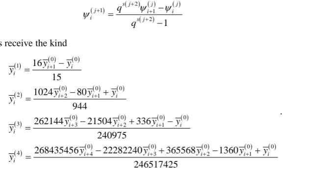
and “direct” formulas receive the kind

( ) ( ) ( )

( ) ( ) ( ) ( )

( ) ( ) ( ) ( ) ( )

( ) ( ) ( ) ( ) ( ) ( )

0 0

1 1

0 0 0

2 2 1

0 0 0 0

3 3 2 1

0 0 0 0 0

4 4 3 2 1

16 15 1024 80

944

262144 21504 336 240975

268435456 22282240 365568 1360 246517425

i i

i

i i i

i

i i i i

i

i i i i i

i

y y

y

y y y

y

y y y y

y

y y y y y

y

+

+ +

+ + +

+ + + +

− =

− +

=

− + −

=

− + − +

=

. (5.5)

The important note: by means of the formula (3.2), it is easy to establish that Simpson’s formula is extrapola-tion of 1-st order of a trapezoidal rule and there is no real necessity to use Simpson’s formula. Let’s remind that application of any schemes of a high exactitude demands high smoothness of functions.

6. Conclusion

(7)

[image:7.595.87.540.99.539.2]

OALibJ | DOI:10.4236/oalib.1102051 7 November 2015 | Volume 2 | e2051 Table 6. Table of extrapolation ( )j

i

y in the point x = 1. The exact magnitude is shown by bold type.

i Ni

( )0 i

y ( )1

i

y ( )2

i

y ( )3

i

y ( )4

i

y

1 2 3.8472 2.612042 2.7205405 2.7182699 2.718281844

2 4 2.9208 2.713759 2.7183054 2.7182818

3 8 2.7655 2.718021 2.7182821

4 16 2.7299 2.718265

5 32 2.7211 2.718281828

∆ .

i ( )0

i

∆ ( )1

i

∆ ( )2

i

∆ ( )3

i

∆

1 0.9263 −0.10172 0.002235 −0.000012

2 0.1553 −0.00426 0.000023

3 0.0356 −0.00024

4 0.0087

δ .

i ( )0

i

δ ( )1

i

δ ( )2

i

δ

1 5.965 23.87 96.14

2 4.369 17.42

3 4.084

γ .

i ( )0

i

γ ( )1

i

γ ( )2

i

γ

1 −0.4912 −0.4916 −0.5022

2 −0.0897 −0.0891

3 −0.0211

References

[1] Richardson, L.F. (1911) The Approximate Arithmetical Solution by Finite Differences of Physical Problems Involving Differential Equations with an Application to the Stress in a Masonry Dam. Philosophical Transactions of the Royal Society of London. Series A, 210, 307-357.

[2] Stetter, H.J. (1973) Analysis of Discretization Methods for Ordinary Differential Equations. (Springer Tracts, Vol. 23). Springer, Berlin, Heidelberg and New York.