Optimal Allocation without Transfer Payments

Munich Personal RePEc Archive

Optimal Allocation without Transfer

Payments

Chakravarty, Surajeet and Kaplan, Todd R.

University of Exeter, University of Exeter and University of Haifa

24 October 2006

Online at

https://mpra.ub.uni-muenchen.de/18481/

Optimal Allocation without Transfer Payments

1

Surajeet Chakravarty

_{Todd R. Kaplan}

March 2009

JEL Classi…cation: C70, D44, D89.

1_{We wish to thank seminar participants at Tel Aviv University, University of Exeter, Third} Congress of the Game Theory Society, Royal Economic Society Meetings in Warwick, Econometrica Summer Meetings Budapest, Electoral Systems and Governance: An Analytic Perspective held at Open University, Israel, and the Dagstuhl fair-division conference. We also wish to thank Ian Gale, Miltos Makris, Gareth Myles, Binya Shitovitz, Eyal Winter, and Shmuel Zamir for helpful comments. Todd Kaplan wishes to thank the Leverhulme Foundation for …nancial support.

2_{School of Business and Economics, University of Exeter, Exeter, UK; email:} [email protected]

Abstract

Often an organization or government must allocate goods without collecting payment in

return. This may pose a di¢cult problem either when agents receiving those goods have private information in regards to their values or needs or when discriminating among agents

using known di¤erences is not a viable option. In this paper, we …nd an optimal mecha-nism to allocate goods when the designer is benevolent. While the designer cannot charge

agents, he can receive a costly but wasteful signal from them. We …nd conditions for which ignoring these costly signals by giving agents equal share (or using lotteries if the goods are

indivisible) is optimal. In other cases, those that send the highest signal should receive the goods; however, we then show that there exist cases where more complicated mechanisms

1

Introduction

One of the basic problems in economics is how to allocate scarce resources or goods. One

of the fundamental di¢culties a-icting such allocation is private information: knowing who desires the goods the most. While markets work well with such allocation, the market is not

always a feasible or desired mechanism for allocation. In case of kidneys it may be unethical to have a market, while in case of sports or concert tickets it may be undesirable to sell the

tickets to the highest bidder.1 _{Finally, with the allocation of charitable goods, it is not only}

undesirable to collect payment in return but those needing it the most are also the least able

to pay for it.2 _{Hence, we often see markets being replaced with other mechanisms.}

One method used is instead of goods being allocated to the person who is willing to pay

the most; they are allocated to who is willing to work the hardest to get them. Sport and concert tickets are given, often using …rst-come …rst-serve mechanism, that is, whoever is

willing to wait the longest before the promoters start selling, gets the right to buy tickets. Allocation of research funds by agencies like National Science Foundation in USA and

Eco-nomic and Social Science Research Council in UK to various universities and individuals are done based on research proposals (where a well-crafted proposal has a higher chance of being

funded). A common feature in these examples is that in order to convey their valuation,

individuals must incur a socially wasteful cost. As with waiting overnight in a long line, generally at least part of this e¤ort is socially wasted.3

Another mechanism that is common with charity, but, surprisingly, also prevalent else-where, is to allocate evenly or randomly using a lottery (among those appearing identical

when classi…ed according to public information).4 _{Often baseball playo¤ tickets are o¤ered}

1_{See Roth et al. (2004) and Roth (2007) for a description of the current method used to allocate kidneys}

and the perceived ethical di¢culties (repugnance) of moving to a market-based system for organ donation and other potentially distasteful transactions. With tickets, there is sometimes a desire for a wider audience. Indeed, the Metropolitan Opera in New York received a several million dollar grant to widen audience by selling prime orchestra tickets for $20 each, 10 percent of their usual price (USA Today,October 5, 2006).

2_{Che and Gale (2006) provide further examples of non-market allocation caused by wealth constrained}

agents.

3_{Without grant money at stake, most researchers would not start a project by writing a detailed, polished}

research proposal. This indicates at least some of the e¤ort is wasted (used ine¢ciently).

via a lottery.5 _{Likewise, NCAA College bowl tickets have a lottery amongst only the season}

ticket holders. Research funds are often handed evenly amongst certain groups or individu-als. For example, most universities hand out …xed research grants to all new sta¤. Allocating

goods equally (ex-ante) has the disadvantage of ignoring any private information, but has the advantage of saving the potential recipients’ e¤ort.

In this paper, we …nd the optimal mechanism to allocate homogeneous, not-necessarily-divisible goods when the bids made by the agents competing for the goods are socially

wasted. Initially, we maximize the social surplus (ex-ante optimality) when values and costs of signalling is private information. We …nd the necessary and su¢cient conditions for when

allocating the goods randomly is optimal. In addition, we …nd the necessary and su¢cient conditions for when distributing the objects to those who work the hardest (a contest)

is optimal. We also …nd cases when other mechanisms can be optimal, such as using a contest but randomly allocating the objects amongst any that meet a certain threshold of

e¤ort (a contest with a bid cap). One interesting result of our paper is that an optimal mechanism does not depend upon scarcity of the goods being allocated. We also show that

our results extend to where a designer may favor one type over another (other interim e¢cient allocations).

The intuition that drives our results are that using signals increases the probability that the good will be allocated to the person who values it the most; however, this naturally also

increases the costs due to signals being wasted. Which mechanism is optimal depends upon this trade-o¤ determined by the distribution of values and signalling costs.

There are many papers examining contests or lotteries, but as opposed to this paper, most study the case where a seller wishes to maximize revenue. Amongst these, Moldovanu and

Sela (2001) study the best way to split prize money in a contest, and Gavious, Moldovanu and Sela (2002) analyze contests, where depending on the nature of the cost function bid

caps may be more pro…table or not. While, Goeree et al. (2005) rank lotteries and contests

mentioned otherwise, everyone is given an equal chance. We call a ra-e a lottery where chances are sold.

5_{More precisely, the price is set below the market clearing price. Since the demand exceeds supply, a}

in fund raising mechanisms and Fullerton and McAfee (1999) model research tournaments

and show that it is optimal to limit the number of participants to two. One paper that does examine allocation with a benevolent designer and thus close in spirit to our paper

is Che and Gale (2006). They …nd that when agents have wealth constraints in a pure market, those that value goods the most cannot necessarily a¤ord them. Hence, sometimes

a random allocation can be superior.6 _{Again with a benevolent designer, Hoppe, Moldovanu}

and Sela (2008), compare match making between two groups (such as men with women)

by pairing those displaying the highest costly signal to that of random matching. Finally, Hartline and Roughgarden (2008) study the bene…t of wasteful signalling in a computer

science application.

In the next section we discuss the allocation problem and convert it into a mechanism

design problem in Section 3. In Section 4, we present the results of our analysis. Finally, in Section 5, we make our …nal remarks and present our conclusions.

2

Allocation Problem

The designer’s problem is to allocateM homogeneous, not-necessarily-divisible goods among

N agents where M < N. The designer is benevolent and wishes to maximize the social

surplus. Each agent i has a privately known type i 2 [0;1] that is drawn independently

from cumulative distribution F. Agenti has valuev( i)for at most one object, wherev( i)

is strictly positive for i >0;continuous and twice di¤erentiable. (If goods are divisible, the

value to agent i is min_fqi;1g v( i) where qi 0 is the fraction of good agent i receives.)

Each agent i is able to send a costly signal xi 2 R+ to the designer. The cost to the

agent of sending signal xi depends upon his type and equalsc(xi) g( i) 0, wherec(xi)is

weakly positive, continuous and strictly increasing whileg( i) is strictly positive for i <1,

6_{Another path to solving the allocation problem is by using psuedo-market systems where exogenously}

continuous and twice di¤erentiable. The functiong( i)captures how the agent’s type a¤ects

the cost of signalling. So if for instance g( i) = i 1, then the higher the type of the agent,

the less costly it is for him to send a high signal. Likewise, if g( i) = i + 1, then the

higher the type of the agent, the more costly it is for him to send a high signal. When g( i)

depends upon i;the designer is able to see the signalxi, but does not know the agent’s cost

of sending the signal. For instance, if the signal is standing in line xi hours, the designer is

able to see how long the agent stands in line, but is unable to determine the (opportunity)

cost to the agent.

Following Milgrom (2004, page 111), without loss of generality we can rewrite our problem

using the uniform distribution on [0;1]in place ofF.7 _{Finally, we assume thatv(}

i)=g( i)is

weakly increasing for0< i <1.8 This can be interpreted as higher the type, the higher the

maximal willingness to send a signal for the object.9 _{This is equivalent to the assumption}

that v0₍

i)=v( i) g0( i)=g( i) for 0 < i < 1. This condition assures that if an agent of

type i is willing to send signal x to have a certain chance of receiving the object then all

agents with typesei i will also be willing to send that signal for the same chance (single

crossing).10 _{We also assume that v; g are analytic.}

After the agents send costly signals, the designer receives these signals (x1; : : : ; xN) and

uses them to allocate the M goods by rule a : RN

+ ![0;1]N where P

iai(x1; : : : ; xN) M

guarantees feasibility. (Note that ai indicates the probability that agenti receives the good

when the goods are indivisible and the fraction of the good received.)11 _{DenoteAas the set} 7_{By having drawn from an arbitrary distribution withvandgfunctions of ;we have a extra degree of}

freedom. By assuming a uniform distribution, we eliminate this extra degree of freedom and gain simplicity of the expressions in the paper. Also by doing so, we are able to continue to treatv( )andg( )even-handedly (not write one in terms of the other).

8_{This is fairly innocuous since we can always reorder v and g to obtain continuous functions that do}

satisfy this condition (and approximate them using twice di¤erentiable functions).

9_{The maximal willingness m is such that v( ) g( )m = 0 or m = v( )=g( ). Note m is in terms of}

cost, that is, one would be willing to send a signalxin order to receive the object if c(x) m: With this interpretation it is again clear one can reorder types to havev=g weakly increasing.

10_{Let us call the chance of receiving the object W (we make use of this notation later in the paper). An}

agent of type i will be willing to send a signal xto receive the object with that chance would so if the

expected payo¤W v( i) c(x) g( i) 0:The derivative of this payo¤ w.r.t. i isW v0( i) c(x) g0( i):

From the inequality (and that v is strictly positive) we have W c(x) g( i)=v( i): This shows that the

derivative is larger thanc(x)[(g( i)=v( i)) v0( i) g0( i)]of which in turn is larger than zero.

of feasible allocation rules. Given allocation rulea, the agents form a Bayes-Nash equilibrium

by choosing a strategy xi( i; a) to maximize their expected surplus given the strategies of

other agents. The designer’s problem is to choose rule a to maximize the equilibrium social

surplus of the agents given the future Bayes-Nash equilibria of the agents, that is, the designer solves

max

a2A

X

i

E[v( i) ai(x1( 1; a); : : : ; xN( N; a)) c(xi( i; a)) g( i)]:

3

Mechanism Design Problem

For simplicity of analysis we will invoke the revelation principle and look at direct

mecha-nisms where each agent i sends a costless (but not necessarily truthful) signal ei.12 Given

the set of signals _fe1; : : : ;eNg, the mechanism gives an object to agent i with probability

Wi(e1; : : : ;ei; : : : ;eN). (Under divisibility, this will represent the fraction good that agent i

receives.)13 _{Likewise, the mechanism charges agentian amounte}

i(ei). Note that this charge

depends only onei. Feasibility requires

X

iWi(e1; : : : ;eN) M:Although the agent incurs

a cost ei(ei) g( i), the designer does not receive any bene…t from the signal ei; that is, the

cost actually incurred by the agent is wasted. The mechanism is truthful if it is incentive compatible (IC) to report truthfully and individually rational (IR) to participate. Once we

solve for the optimal direct mechanism, then we can implement the solution by choosing an appropriate allocation rule, that is by settingai(x) = Wi(e11(c(x1)); : : : ; eN1(c(xN))), we

have c(xi( i; a)) =ei( i): Notice that this can be implemented since ei( i) does not depend

upon j (j 6=i).

Now by limiting ourselves to symmetric mechanisms, we can denote W(ei) as the

prob-ability of agent i receiving an object with message ei when everyone else reports truthfully

the equivalent to giving the agent measure one and disposing of the excess.

12_{Note that there is no bene…t to having a sequential mechanism such as in Crémer et al. (2009) since all}

parties know their private information initally.

13_{A lottery would allocate objects with probability W}

i(e1; : : : ;eN) = M=N. A contest with M = 1

would allocate objects according to Wi(e1; : : : ;eN)equals 0 ifei <maxfe1; : : : ;eNg or equals1=#if ei=

and e(ei)as the expected cost given that everyone else reports truthfully.14;15 For simplicity

of notation, we drop the i subscript. Both W(e) and e(e) are assumed to be increasing in e. Now an agent of type reporting e (with all others reporting truthfully) has payo¤

( ;e) W(e)v( ) e(e) g( ). The agent solvesmax_e ( ;e)which in a truthful mechanism should equal ( ; ).

The designer chooses W(e) and e(e) to maximize N E[ ( ; )] = N E[W( ) v( )

e( ) g( )] subject to W( ) being consistent with feasibility, IC ( ( ; ) ( ;e)) and IR ( ( ; ) 0). Before getting to our results, in the following lemma we simplify the designer’s problem by eliminating from the problem, the IC and IR constraints as well as the choice of

e( ):

Lemma 1 The designer’s problem reduces to choosingW( )that is increasing and consistent with feasibility in such a way to maximize the social surplus given by

N

Z 1

0

W( ) v( )

g( )

0 Z 1

g(^)d^ d +N W(0)v(0)

g(0)

Z 1

0

g( )d N W(1)`1; (1)

where `1 = lim !1 n

v( )

g( ) R1

g(^)d^ v( ) (1 )o.

Proof. See the Appendix.

Notice that as one may expect increasing v( ) to v( ) increases surplus by factor :

Also, somewhat less obvious, increasing g( ) to g( ) does not alter the surplus. This is for the same reason that our cost function, c(x); does not appear in the surplus. Namely, if agents have proportionately lower waiting costs, they will simply dissipate the gains by proportionately increasing the cost of e¤ort.

14_{Note it is not optimal to restrict the number of participants as opposed to other environments where the}

designer values the signals such as Fullerton and McAfee (1999), indicative that our symmetric assumption is not crucial.

15_{Note that in order to be able to determine the allocation rule, we would need to decomposeW( ) into}

Wi(e1; : : : ;eN):This is not a problem since any mechanism described byW( )that is feasible with increasing

W( ) can be decomposed into a mechanism Wi(e1; : : : ;eN) that is symmetric and satis…es monotonicity:

if ei > e

0

i then Wi(e1; : : : ;ei; : : : ;eN) Wi(e1; : : : ;e

0

i; : : : ;eN). Likewise, any mechanism that satis…es

4

Results

4.1

Optimal Mechanism

We now use the simpli…ed designer’s problem to solve for an optimal mechanism in a manner

similar to Myerson (1981).16 _{Denote the surplus per object from running a lottery for N}

agents as S` (that is, equation (1) with W( ) = 1=N): Also, denote

z( ) =

8 > > > < > > > :

0 if = 0;

R 0

v(e)

g(e)

0 R₁

e g(^)d^ de+vg(0)(0) R1

0 g(e)de if <1;

S` if = 1:

The expressionz( )= represents the average virtual surplus of all types from0to :17 Hence,

z0_{( ) =} v(e)

g(e)

0 R₁

e g(^)d^ is the virtual surplus for type . Note that the end points of 0

and 1contain what can be thought of as a …xed virtual surplus. While this is non-standard, one can understand this better by using the analogy of a cost function c(y) where c0_{(y) is}

the marginal cost,c(y)=y is the average cost, and limy&0c(y) the …xed cost.18

Let C( ) be the convex envelope of z( ), that is,C( ) =Conv(z( )) where

Conv(z( )) = inf

r; 1; 2

rz( 1) + (1 r)z( 2)

s.t. r; 1; 2 2 [0;1] and r 1+ (1 r) 2 = :

Since _C is convex, _C00 _0.

Proposition 1 An optimal mechanism has the following allocation: the interval [0;1] can be divided into regions where _C00_{( ) > 0 (a contest) or when C}00_{( ) = 0 (a lottery). Goods}

16_{There is a unique ex-ante optimal allocation if the set f 2[0;1]j d} v( )

g( )

0 R₁

g(^)d^ =d = 0g has measure 0.

17_{Virtual surplus is the surplus generated by giving the object to someone of type taking into account the}

full cost this has on incentives. Namely, the cost to designer of keeping the other (higher) types truthtelling rather than pretending to be a lower type.

18_{We may havelim}

are allocated sequentially. If the highest type falls within a contest region, then the agent

of that type receives the good, otherwise there is a lottery among all agents whose types fall

within that region. That agent is removed and the process is repeated until all goods have

been allocated.19

Proof. See the Appendix.

The required monotonicity of the W( ) function causes the allocation to be in regions of contests and lotteries. If a designer needing to allocate one object between two agents receives signals of 1 and 2; where 1 > 2, then the designer can either give the object

to the player with 1 or randomly allocate the object between both players. If the designer

receives signals b1 and 2; where 1 >b1 > 2 and would choose a lottery between 1 and

2, then he should also choose a lottery betweenb1 and 2: If the designer receives signals bb₁ and 2;where bb1 > 1 > 2 and would choose 1 over 2, then he should alsobb1 over 2:

(We explain this further in the examples).

In order to see why the convex envelope _C yields the optimal allocation, start with

allocating objects according to the highest type. Take the graph ofz( ):If there is a region, [ 1, 2];that is concave (decreasing slope) on[ 1, 2];then allocating this by the highest type

would not yield the highest revenue since one would more likely be giving it to someone with a lower virtual surplus (lower slope of z). Replacing this with a lottery on [ 1, 2]will yield

higher surplus.20 _{The average virtual surplus in that region is (z(}

2) z( 1))=( 2 1):

This is equal to the slope of the line from ( 1; z( 1))to ( 2; z( 2))on the graph of z( ). We

can thus replace region with on a new z( ) with a line between those points. Now, it is worthwhile to expand any regions by including the type at 2 to the lottery on [ 1; 2] if

slope ofz( 2)at 2 is smaller than the slope of the line from( 1; z( 1))to( 2; z( 2)). Thus,

19_When`

1<0;we de…ne = 1as a contest region.

20_Iff

1 (the probability of receiving an object) is strictly increasing andf2(the virtual surplus) is strictly decreasing, then R 2

1 f1( )f2( )d <

R ₂

1f1( )d 2 1

R 2

1 f2( )d . This holds since

R ₂

1 f1( )d

2 1 is the

av-erage of f1 on [ 1; 2]: The inequality now becomes R 2

1 (f1( ) )f2( )d < 0: De…ne such that = f1( ): We now have R 2

1 (f1( ) )f2( )d =

R

1 (f1( ) )f2( )d +

R 2_(f

1( ) )f2( )d <

R

1 (f1( ) )f2( )d +

R 2_(f

the region should be expanded until the average virtual surplus in the lottery region stops

decreasing. Graphically, this is until the line from ( 1; z( 1))to the end of the lottery stops

decreasing in slope.21 _{By repeating this process, we arrive at the convex envelope C which}

generates the optimal allocation.

Now making use of Proposition 1, we …nd which mechanisms will result in the optimal

allocation.

4.2

When a Lottery is Optimal

We now with help of Proposition 1, we can specify necessary and su¢cient conditions for a

lottery to be optimal.

Proposition 2 A lottery is an optimal mechanism if and only if for all the average virtual

surplus up to is greater than the (overall) average virtual surplus, that is, z( )= z(1)

for all :

Proof. The mechanism presented in Proposition 1 will be a lottery if and only ifC00_{( ) = 0}

for all : This will happen if and only if convex envelope is obtained from the endpoints,

that is, C( ) = (1 )z(0) + z(1) = z(1): This happens if and only ifz( ) z(1):

Example 1 When N = 2, M = 1; which has higher surplus: (a) holding one lottery or (b) holding a lottery among types below and a lottery among types above ?

The overall lottery yields higher surplus over the two lotteries if and only if z(1)

2 z( )

+ (1 2) z(1)₁ z( ) = (1 + )z(1) z( ); yielding z( ) z(1). We see this in agreement with Proposition 2.

While it is useful to have necessary and su¢cient conditions for a lottery to be optimal,

we …nd it also useful to examine particular su¢cient conditions as well.

21_{The beginning = 0, can be thought of as a degenerate lottery region. If} v(0)

g(0)

R1

Proposition 3 (i) If v_g( )_{( )} 00 0, then a lottery is optimal.

(ii) If v(1) is bounded and g(1) > 0, then there exists an > 0 where for environment g;

b

v( ); where _bv( ) =v( ) + g( ); a lottery will be the optimal mechanism.22

Proof. First, we prove (i). If v( )

g( )

0 R₁

g(^)d^ is weakly decreasing and`1 0, then

a lottery is an optimal mechanism. Begin by looking at the …rst part of the expression

in Lemma 1. Since the part inside the integral (not considering W( )) is decreasing, the integral is maximized with a lottery (‡at W( )). Now notice that the second part of the expression in Lemma 1 is maximized by maximizingW(0);this happens also with a lottery (since W must be weakly increasing). Finally, since `1 0; the third part is maximized by

minimizing W(1), which also happens with a lottery. Now notice that

d[ v_g( )_{( )} 0 R1g(^)d^

d =

v( )

g( )

00 Z 1

g(^)d^ v( ) g( )

0

g( ):

By the mean value theorem, we have

v( )

g( )

00

(1 )g( ( )) v( )

g( )

0

g( )

where ( )is between and 1. If v( )

g( )

00

0, then this expression is negative. If v( )

g( )

00

0; then v(1)

g(1) is bounded. If v(1) is also bounded, then `1 = 0: If v(1) is unbounded, then for

v(1)

g(1) to be bounded we must haveg( ) increasing as approaches 1. If so, by the mean value

theorem, v( )

g( ) R1

g(^)d^ v( ) (1 ) 0 and hence `1 0.

The proof of part (ii) is in the Appendix.

Note that part (i) that a lottery is optimal if v=g is weakly concave. From the surplus, slope ofv=g does not a¤ect the decision upon which mechanism to employ. However, if this

slope is increasing, it becomes increasingly expensive in terms of value for the high types

22_{It is also possible to show that if(1 )v}0_{( )is decreasing in andg}0_{( ) 0;then a lottery is socially}

to signal. In this case, the messages made by the higher-value agents are too costly for

the society to waste and therefore it is better to run a lottery, that is, allocate the good randomly.23 _{While the proof of part (ii) is not particularly straightforward, the intuition of}

the result is clear. Since bv( )=g( ) = v( )=g( ) + ; a larger makes the di¤erent types relatively close in terms of v( )=g( ). Hence, when the di¤erences between types become relatively smaller, that is, a larger part of the value is common, a lottery would be the optimal mechanism. We now see that the su¢cient conditions can be useful in …nding examples where

a lottery is optimal.

Example 2 N = 2, M = 1; v( ) = ; and g( ) = 1:

In this case, v( )

g( )

00

= 0. Thus, the social planner does better by running a lottery, with surplus R₀1(1 )d = 1₂, than a contest, with surplus 2R₀1(1 ) d = 1₃, (or any other mechanism).

This contrasts with a mechanism that maximizes revenue when payments can be collected.

Namely, types < 1

2 are excluded and the agent with the highest ( 1

2)receives the object.

Example 3 v( ) = ( +c) and g( ) = ( +c) where ; c; >0 and 0< 1:

In this case, v( )

g( )

00

= 2_{( )( 1) ( +c)} 2 _{0. Hence, a lottery is}

socially optimal.

This is a generalization of the previous example.24 _{Notice that a lottery can be optimal}

when g0_{( )<0 org}0_{( ) >0.}

23_{With possibility of costless messages, a lottery is only the unique optimal mechanism among monotonic}

mechanisms (as described in footnote 15). For instance, whenN= 2,M = 1, one can ask players to send a costless signalsi of their types. Ifsi > sj then only ifsi sj <0:5, the mechanism would allocate it to i.

If players truth tell, the expected probability of winning will be the same. Monotonicity is violated since if

s2= 0:8;player 1 wins with a signal ofs1= 0:1, but loses with a signal ofs1= 0:4:

24_{When c = 0; a lottery is still socially optimal even though our assumption that g(0) >0 is violated.}

4.3

When a Contest is Optimal

We can also use Proposition 1 to specify the necessary and su¢cient conditions for a contest

to be optimal.25

Proposition 4 A contest is an optimal mechanism if and only if v_g( )_{( )} 0 R1g(^)d^ is weakly increasing, v(0) = 0 and `1 0:

Proof. This follows from Proposition 1. It will be a contest if and only if _C00_{( )>0 for}

all : This will happen if and only if C( ) = z( ): This happens if and only iflim &0z( ) =

z(0), lim %1z( ) z(1); and z00( ) 0: Well, z00( ) 0 i¤ v(

e)

g(e)

0 R

1

e g(^)d^ is weakly

increasing, lim &0z( ) =z(0) i¤ v(0) = 0; and lim %1z( ) z(1) i¤ `1 0:

Corollary 1 (i) For a contest to be optimal, we must have v_g( )_{( )} 00 0 everywhere. (ii) For a contest to be optimal, either v(1) needs to be unbounded or g(1) must equal 0:

Proof. From the proof of Proposition 2 (i), we have

d[ v_g( )_{( )} 0 R1g(^)d^

d =

v( )

g( )

00

(1 )g( ( )) v( )

g( )

0

g( ):

From Proposition 4, this must be weakly positive for a contest to be optimal. This can only

happen if v( )

g( )

00

0 everywhere.

From the proof of Proposition 2 (ii), ifv(1)is bounded andg(1)>0, thenlim !1 v_g( )_{( )}

0 R₁

g(^)d^ =

0: This shows that v( )

g( )

0 R

1

g(^)d^ cannot be weakly increasing.

We now provide two examples where a contest is the best way to allocate a good. In the …rst case, v is unbounded. In the second case, g(1) = 0.

25_{Such conditions would require that the designer would allocate to the objects to the agent with the}

Example 4 N = 2, M = 1, v( ) = ₍₁ 2₎0:5 2; and g( ) = 1.

Notice that v( )

g( )

0 R₁

g(^)d^ = ₍₁ 1₎0:5 is increasing on [0;1] and `1 = 0 (since g is

constant). Surplus from a pure contest is 2R₀1 ₍₁ 1₎0:5 d = 2 2

3 and is more than that from a

lottery R₀1 1

(1 )0:5d = 2. Here, the contest does best.

Example 5 N = 2, M = 1; v( ) = ; and g( ) = (1 )2_:

Here v( )

g( )

0 R₁

g(^)d^ = (1 + )1₃ which is increasing in ; v(0) = 0 and `1 = 0:

Remark 1 The optimal mechanism depends upon v and g, not just v=g.

We see this by means of the following example which has the same v=g ratio as the previous example but instead of a contest being optimal, a lottery is optimal.

Example 6 N = 2, M = 1; v( ) = (1 ); and g( ) = (1 )3_:

Here,R₀ v(e)

g(e)

0 R₁

e g(^)d^ de=

R

0 1 e

2 ₁

4de= 4 3

12:Sincev(0) = 0;

v(0)

g(0) R1

0 g(^)d^ =

0. The expected surplus of running a lottery is S` =

R1

0 (1 )d =

1

6: Since 4 3

12 1 6

for all 2[0;1]; a lottery is optimal.

4.4

When More Complicated Mechanisms Are Optimal

There are still possibilities under Proposition 1 when neither a lottery or contest is optimal.

Remark 2 Under certain conditions, a more complicated mechanism can be optimal such

as

(i) a contest with a bid cap,

(ii) a lottery among low types but a contest for high types,

(iii) several regions where each region is of contest or lottery.

lottery, when all values are low, followed by a contest for higher values is optimal. Finally,

in example 9, we show that a contest followed by a lottery and then again followed by a contest is the optimal mechanism. Note that in all the examples the main intuition for the

use of a particular mechanism, is if the virtual surplus increases or falls. If the virtual surplus increases then it means that e¢ciency increases with a non-cooperative bidding mechanism

while if the surplus falls a random allocation is better.

Example 7 N = 2; M = 1; v( ) = ₂2 and g( ) = 1:

Notice here that v( )

g( )

0 R

1

g(^)d^ = (1 )increases and then decreases in . Con-sider the following allocation where 1 and 2 denote the types of the agents. If 1; 2 ;

then the good is allocated randomly, otherwise whoever has the higher gets the good. Such

an allocation results from running a contest with an appropriate bid cap. Under such an allo-cation the social surplus isNR₀ W( ) [ (1 )]d +NR1 (1 ) P d :A bid cap allows us to implement the above allocation by choosing , the probability of winning with is

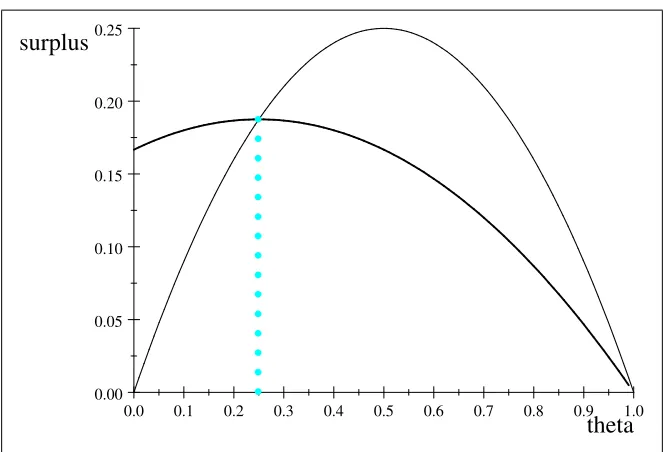
(1+ )=2:Surplus is then2R₀ (1 )2 2d +2R1(1 )(1+ ) d = 1₃ 2+ 3 1₃ 4+1₃ which achieves its maximum of 0:36849 at = 1=4:26

Examine the thin line in Figure 1. This represents the virtual surplus of giving the object

to an agent of type . For all , it is also worthwhile to give the object than not to give the object. Notice that for points to the right of the graph, such as = 0:9 and = 0:8; one would prefer to give the object to the agent with lower : However, with the restriction in probability, the designer can at most keep the probability of receiving the object the same

(holding a lottery). While the surplus reaches the peak at = 0:5; we would still want to hold a lottery between someone with someone with = 0:5and someone with = 0:4;since under the increasing probability restriction, we must choose between either holding a lottery amongst someone with = 0:4 and all those with 0:5 or always giving the object to all those with 0:5 over someone with = 0:4:27 This leads us to the thick line in the graph.

26_{The equivalent bid cap ofxsetsc(x) = 0:00716:}

27_{This is necessary to be consistent with monotonicity as describe in footnote 15. For instance, if we choose}

someone with = 0:5 over someone with = 0:4 while choosing someone with = 0:4 over someone with

This line represents the average virtual surplus of all 0 _{: The optimal mechanism will}

weigh this average against the virtual surplus of :When the surplus of is higher, then will be added to the lottery. When the average above is higher, then higher will be preferred

as in a contest. The average surplus above is hR1b(1 b)dbi=(1 ) = 1

6(1 )(1 + 2 ).

This equals the virtual surplus when 1

6(1 )(1 + 2 ) = (1 ) or when = 1=4;

con…rming the above.

Thus far, we have presented the mechanism in terms of :Now, we demonstrate how this

would work in terms of bidsx. To do so, we must …rst calculate the expected e¤ort an agent of type must expend in the optimal mechanism. The probability of getting an object with

type <1=4is just the probability that the other agent has a lower type :For 1=4it is the probability that the other agent has a type less than 1=4plus half the chance otherwise, totalling5=8. Thus,

Wi( ) =

8 < :

if <1=4;

5

8 otherwise.

We can now substitute this into equation (3), yielding28

ei( ) =

Z

0

Wi0(^)

^2 2d^ =

8 < :

3

6 if <1=4;

(1 4) 3 6 + 3 8 (1 4) 2 2 = 11 768 otherwise.

Finally, c(x( )) = ei( ): This implies that the bid cap x will be set such that c(x ) =

ei( ) = ₇₆₈11: If c is linear, this is the bid cap. Notice that this is incentive compatible since

the highest bid before the cap, lim _%1

4x( ) = lim % 1

4 ei( ) =

(1 4)

3

6 =

1

384. The expected

pro…t of an agent with = 1=4 bidding 1 384 is 1 4 (1 4) 2 2 1 384 = 1

192; while bidding at the cap

of 11 768 yields 5 8 (1 4) 2 2 11 768 = 1

192: An agent with a higher , gains more from winning, while

an agent with a lower gains less from winning. Since bidding at the bid cap wins with higher probability, all agents with < 1=4 prefer bidding beneath the bid cap and agents with 1=4 prefer bidding at the bid cap.

28_{Note that over the discrete jump inW}

i( ); we make use of Dirac-Delta functions to obtain our results

0.0 0.1 0.2 0.3 0.4 0.5 0.6 0.7 0.8 0.9 1.0 0.00

0.05 0.10 0.15 0.20 0.25

theta surplus

Figure 1: In example 7, the winner is by highest signal and after a threshold = 1=4, by lottery. Thin line is virtual surplus and thick line is average virtual surplus above .

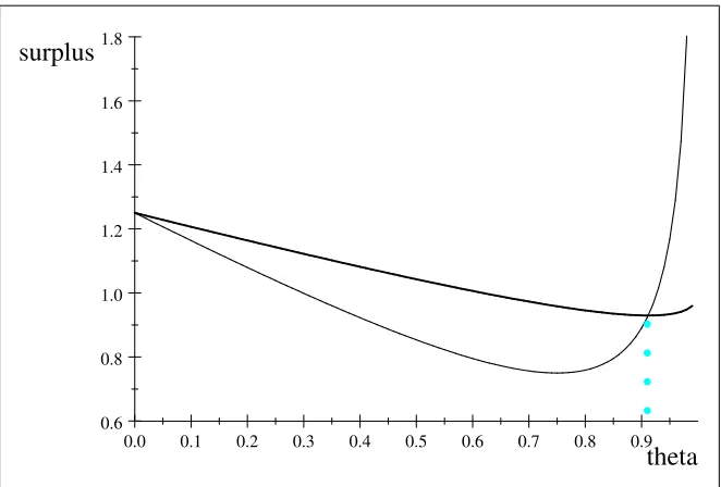
Example 8 N = 2; M = 1; v( ) = 1

2p(1 )+ 1

2 and g( ) = 1:

Here v( )

g( )

0 R₁

g(^)d^ = (1 ) 0:25

(1 )1:5 + 1 : It …rst decreases until = 0:75; and

then increases until = 1. Consider the following allocation where 1 and 2 denote the

types of the agents. If 1; 2 ;then the good is allocated randomly, otherwise whichever

is higher gets the good. Such an allocation results from running a contest with a minimum

bid and allocating the good randomly if no one meets the minimum bid. From this, the social surplus is R₀ h(1 ) 0:25

(1 )1:5 + 1

i

d +NR1 h(1 ) 0:25 (1 )1:5 + 1

i

d : We will now

see that this is the optimal mechanism under the probability limitation.

In Figure 2, as before, the thin line in the graph represents the virtual surplus of giving

the object to an agent of type . Again, for all , it is also worthwhile to give the object than not to give the object. Notice that now for points to the left of the graph, such as = 0:2 and = 0:1; a designer prefers to give the object to the agent with lower : Hence, under the probability restriction, the designer would choose a lottery for those points. While the

to those in example 7. Namely, since under the increasing probability restriction, we need to

make the choice between holding a lottery amongst someone with = 0:8and all those with 0:75or always giving the object to someone with = 0:8over all those with 0:75:29

This leads us to the thick line in the graph that represents the average virtual surplus of all 0 _{:The optimal mechanism will weigh this average against the virtual surplus of :If}

the surplus of is higher, then will be preferred. When the average below is higher, then will be added to the lottery. This crossing point is at = 0:9117:As in example 7, we can use equation (3) to determine the minimum bid to be included in the all-pay auction. Since in the lottery phase, when < ; W0_{( ) = 0 we have e( ) =} R _W0_(^)v(^)

g(^)d^ = 0: Going

from the lottery to the all-pay auction the jump in probability is =2: Thus, the jump in e¤ort must be lim & e( ) = ₂ v_g(₍ )₎ = ₂ 1

2p(1 ) + = 1:1826: This should equal the

cost of bidding for the agent with type , hence c(x( )) = 1:1826: If c(x) =x2_{; then the}

minimum bid should bep1:1826 = 1:0875:

0.0 0.1 0.2 0.3 0.4 0.5 0.6 0.7 0.8 0.9

0.6 0.8 1.0 1.2 1.4 1.6 1.8

theta surplus

Figure 2: In example 8, the winner is by lottery, and then by highest signal. Thin line is

virtual surplus and thick line is average virtual surplus above :

29 _{Otherwise, monotonicity from footnote 15 is broken. For instance, if we choose someone with =}

0:2 over someone with = 0:8 while choosing someone with = 0:8 over someone with = 0:75; then

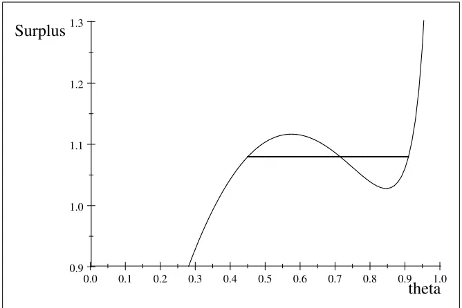
Example 9 N = 2, M = 1; v( ) = ₂₍₁ 1₎0:5 +3₂ 2 1₂ and g( ) = 1:

Here v_g( )_{( )} 0 R1g(^)d^ = (1 ) 0:25

(1 )1:5 + 3 . This …rst increases, then decreases,

and then again increases till = 1. In this case, the following mechanism is optimal, where the social planner …rst runs an all-pay auction then a lottery and then runs an all-pay auction for the high value agents. This yields the following allocation: 1 and 2 denote the types

of the agents. If 1; 2 are in[0:45;0:91], then the good is allocated randomly. Otherwise, it

is allocated to the one with the highest : Note that from = 0:45 to = 0:91 the social planner will run a lottery and in the rest of the range a contest will be used. Therefore, the social surplus is

2

Z 0:45

0

(1 ) 0:25

(1 )1:5 + 3 d + Z 0:91

0:45

(1 ) 0:25

(1 )1:5 + 3 (0:91 0:45) d

+2

Z 1

0:91

(1 ) 0:25

(1 )1:5 + 3 d :

This is a combination of our two previous examples with the lottery range in the middle.

Denote the lottery range from a to b. We must compare the average virtual surplus of

those in the range to those out of the range. We would prefer a in[ a, b] to those below a

if the average surplus is higher than the surplus of all those below and prefer those above b

if the average surplus is lower than the surplus of all these values. Since the virtual surplus

is increasing (and continuous) outside of this range, this can only happen if the average virtual surplus is equal to the virtual surplus on both ends: R b

a s( )d =s( a) =s( b): We

see this in Figure 3. Again, the thin line is the virtual surplus. Here, the thick line helps to demonstrate the range of types where a lottery should be used. With this line, both

endpoints have the same virtual surplus. This virtual surplus should also equal the average virtual surplus in the range of the thick line. In order for this to happen, the area above it

and below the thin line and below it and above the thin line should cancel (be equal). As with examples 7 and 8, we can determine the mechanism in regards to an auction.

x and x will count only as much as x. These can be determined in a similar way as in

examples 7 and 8.

0.0 0.1 0.2 0.3 0.4 0.5 0.6 0.7 0.8 0.9 1.0

0.9 1.0 1.1 1.2 1.3

theta Surplus

Figure 3: In example 9, the winner is by highest signal except for the interval

2[0:45;0:91] Thin line is virtual surplus and thick line is the interval [0:45;0:91]: The area below the thin line and above the thick line is equal to the area above the thin line

and below the thick line.

We observe in numerous instances where goods are allocated by one of the more compli-cated methods of examples 7 to 9, that is, a method beyond a straight lottery or contest. For

instance, the way example 7 could work in practice, is to allocate tickets for an event by hav-ing a lottery for anyone that waitsx hours for tickets and if there are tickets left after that,

allocate the tickets through lottery. Another illustration of this is the ticket distribution by All England Tennis and Croquet Club for the Wimbledon tennis tournament. The club …rst

holds a lottery to allocate the tickets almost six months before the Wimbledon tournament and then gives them away in …rst come …rst serve basis or person willing to stand longest in

the queue. (We presume that buying tickets six-months prior takes more e¤ort.) We see a system like example 8 with the distribution of entries in the New York marathon.30 _Those

30_{Some may be surprised to discover that the right to run in the major marathons needs to be rationed.}

that put in greater e¤ort can qualify automatically (by completing a number of sanctioned

races or making a qualifying time), remaining entries are distributed by a lottery system. Finally, in example 9, we see where it is optimal to run a contest …rst, and then allocate

the good randomly and for the higher values again run a contest. One possible example of this is admissions to top US universities among students with high test scores. Writing an

essay is part of the application. As most lecturers know, most essays are indistinguishable in level. A few good ones stand out as well as a few bad ones. It is possible that an admissions

o¢cer would …rst admit the good essays and then randomly select among the middle pile. If there are still slots left, the o¢cer may start to o¤er admissions to the top of the lower

group. Similarly, there are more students that apply to Oxford or Cambridge Universities with the highest score on the admissions tests (three As in the A-level exams) than places.

To select students, interviews are held. We can interpret the interviews (where preparation can help) as the socially wasteful but necessary to signal the type of the students.

4.5

Scarcity

An important question is whether scarcity of goods (the number of goods relative to the number of agents) favors one mechanism over another. To answer this question, we must

…rst …nd a way to compare mechanisms across environments. We do so by the following de…nition.

De…nition 1 Two mechanisms are said to be equivalent if their W functions have the same

regions where they are strictly increasing, that is, a mechanism characterized by Wa is

equiv-alent to one characterized by Wb if for all 2 > 1; we have Wa( 2)> Wa( 1)()Wb( 2)>

Wb( 1).

We can now use the above de…nition to show that an optimal mechanism does not depend upon the scarcity of the good.

Proposition 5 For any mechanism that is optimal in environment (v; g; M; N) (and de-scribed by Proposition 1) there is an equivalent mechanism that is an optimal mechanism in

environment (v; g;M ;c Nb). However, which of two equivalent non-optimal mechanisms yield higher social surplus may depend upon M or N.

Proof. DenoteCa as theC function used to generate the mechanism (via Proposition 1)

for environment(v; g; M; N)resulting in theW function,Wa. Notice thatWa( 2)> Wa( 1)

if and only if Ca( 2) > Ca( 1). Now notice that C functions are independent of M or N

(they depend only on v and g). Hence, for environment (v; g;M ;c Nb) the _C function would equalCaand hence theW function,Wb, would have the property thatWa( 2)> Wa( 1)()

Wb( 2)> Wb( 1).

We will now show the second part of the proposition. We do so by means of an example showing that in comparing two non-optimal mechanisms which is higher changes in either

M orN. More speci…cally, a lottery is optimal whenM = 1 and N = 3; however, a contest is optimal either when M = 2 and N = 3 or M = 1 and N = 2. The details are as follows: g( ) = 1 and v( ) = ; yielding virtual surplus of (1 ): The social surplus with a contest with one object,M = 1;is N

(N+ )(N+ +1). The surplus with a contest with two

objects,M = 2;is (3N+ 3)N

(N+ )(N+ +1)(N+ 1). The surplus with a lottery is

M

(1+ )(2+ ) (independent

of N): Take = 5=4. When we haveN = 2 and M = 1, the surplus for the contest, 0.1447;

is greater than that of a lottery, 0.13675, however whenN = 3 and M = 1; this is reversed, with surplus from contest, 0.1344, which is now smaller than that of a lottery. Finally, when

we move to N = 3 and M = 2, the contest is again better than a lottery, with contest surplus, 0.299, and lottery surplus, 0.273.

Taylor et al. (2003) and Koh et al. (2006) analyze allocation through lotteries and queues, and …nd that lotteries are more e¢cient in comparison to waiting line auctions if the time

valuation are less varied and objects are scarce. This may be surprising compared to the …rst part of the proposition, however the second part shows how our paper is consistent.

compared only two di¤erent mechanisms.31

4.6

Other Interim-E¢cient Allocations

Up to this point, we have studied ex-ante Pareto-optimal allocations. In such a manner, the designer treats every type with the same ex-ante weight. It is conceivable that the designer

may want to favor some types over others. For instance, a designer may wish to count higher types more (they could be future donors) or lower types more (increasing future interest).

To include such a possibility, we need a set of weights ( ) such that R₀1 ( )d = 1 for which the designer would maximizeN E[ ( ) ( ; )]:This leads to the set interim-e¢cient allocations (see Ledyard and Palfrey, 2007). Observe that for equal weights, ( ) = 1; we have our original case of an ex-ante e¢cient allocation.

Proposition 6 A ( ) interim-e¢cient allocation for environment v( ) and g( ) is given by Proposition 1 where _C( ) is de…ned using _bv( ) ( )v( ) and _bg( ) ( )g( ) instead of v( ) and g( ):

Proof. In order for this proposition to hold, we need to show two problems yield the

same solution: (A) choosingW( )and e( )to maximize N E[ ( ) ( ; )] subject to W( ) being consistent with feasibility, IC and IR constraints and (B) choosing W( ) and e( ) to maximize N E[_b( ; )] (where b( ; ) W( ) _bv( ) e( ) _bg( )) is subject toW( ) being consistent with feasibility, IC and IR constraints (with bv( ) and bg( )).

Notice thatN E[ ( ) ( ; )] =N E[W( ) ( )v( ) e( ) ( )g( )] =N E[_b( ; )]. Thus, the objective function is the same. We now show that any allocation that satis…es IC

and IR constraints forvb( )and bg( ) will also satisfy IC and IR constraints forv( ) and g( ) and vice-versa.

De…ne b( ;e) W(e) _bv( ) e(e) _bg( ): Now b( ; ) _b( ;e) ₍₎ ( ; ) ( ;e) because b( ;e) = W(e) ( )v( ) e(e) ( )g( ) = ( ) ( ;e): Likewise, b( ; ) 0

31_{Other notable earlier papers on waiting-line auctions include Barzel (1974), Holt and Sherman (1982)}

() ( ; ) 0. Feasibility is also the same. Since the objective and constraints are the same, the solution must be the same. (Since bv( )=_bg( ) = v( )=g( ); our assumption that

v=g is increasing is still su¢cient.)

As we see from the following Corollary, the Proposition expands our results.

Corollary 2 The results of sections 4.1 to 4.5 hold for _bv( ) and _bg( ) in place of v( ) and

g( ):

One result that may seem surprising is that if v( )

g( )

00

0, then a lottery is optimal for any weighting of types. Intuitively, one may expect when higher types are weighted more, then a lottery may not be optimal. However, v( )

g( )

00

0is enough to ensure that the virtual surplus is decreasing for any ( ), since d[

h

(v( )

g( )) 0

(R1 _(^)g(^)d^)i

d =

v( )

g( )

00 R₁

(^)g(^)d^

v( )

g( )

0

( )g( ):

5

Concluding remarks

This paper makes a contribution in the allocation of goods when signalling one’s desire for the good is a wasteful activity. Under such conditions, there is a trade-o¤ between e¢cient

allocation and wasted resources. A mechanism such as a contest, which allocates by the highest signal, will allocate goods to the people who value them the most but the act of

signalling will be wasteful. Allocating an equal share to everyone (or a random allocation by a lottery) saves any waste from signalling, but leads to an ex-post ine¢cient allocation.

This analysis has many additional applications. Contests are also used to grant the Olympic games, where the individual cities submit bids, and part of the bids are often

socially wasted. In the UK, governmental research funds are distributed through two main channels: research councils or quality-related (QR) funding. Research councils allocate funds

to institutions by gathering private signals through research grant applications, for which the paper work can be considered socially wasteful. QR funding allocates funds through publicly

is done through the Research Assessment Exercise, RAE). Our analysis can help design an

appropriate mechanism. If the cost incurred by the institutions to make the case for grants is too high, the government should favour QR funding. Policy research into which system is

best is an important area in which our paper contributes.

Our results also has implications for bidding rings (cartels) in auctions. In this literature,

McAfee and McMillan (1992) …nd an optimal mechanism for collusion that agrees with our results. Namely, if the hazard rate is decreasing, bidders should participate in the auction

non-cooperatively; however, if the hazard rate is increasing, then bidders should bid the reserve price whenever they value the object more than the reserve. In this application, the

cartel’s objective is congruent to that of our designer while the bids are analogous to our wasteful signal. Hence, our results indicate that the McAfee and McMillan results apply more

generally.32 _{Moreover, a connection would show that in many cases the optimal collusive}

policy would be something more complicated such as an increasing bid function that reaches

a peak or bidding the reserve price for low values and then jump to bidding higher values. There are many possible changes to our basic model for which similar analysis could be

used. One change is to relax our key assumption of a wasteful signal to a partial wasteful signals. For instance, an agent of type sending a signal of x may have private value of

sending the signal of c(x)g( ): This means the true waste is only(1 )c(x)g( ); however, as we saw that the cost functionc(x) has no a¤ect on the optimal mechanism, this will also have no a¤ect. If instead there were a public bene…t to such a signal, then the higher the bene…t, the more likely the optimal mechanism would favour contests. We can also partially

relax the assumption on payments to the designer. The necessary element for our analysis to apply is that there is a maximum price that the designer can charge and at this price,

there is an excess demand (as the case with playo¤ tickets). The timing of the signals in our mechanism can also be changed while keeping the same nature of our results. For instance,

a war of attrition can be used to allocate goods in place of a contest. A war of attrition with a time limit can be used in lieu of a contest with a bid cap.

32_{There is still the discrepancy of the all-pay nature of our signals versus the …rst-price payments in an}

While in this paper, we examined only the case where each agent has one of two possible

allocations: with an object or without an object, we can apply this in any case with two possible outcomes. Think of the case where a course is o¤ered twice and students have to

decide which time they want to be scheduled for (with all students being assigned to one of the two slots). If there is an excess demand for one of the time slots, then one can use our

analysis to determine how to allocate the slots to the students demanding the popular time slot. (All students demanding the less popular slot will get it.)

A natural extension for our paper would be to consider several types of goods. Doing so would make it possible to explore a link to papers on pseudo-markets (markets using points

rather than money), except we will optimize the method for obtaining points as a function of e¤ort (better grades yield more points in course markets). An exogenous allocation of

points is similar to a lottery while points solely as a function of e¤ort is like a contest. Fairness issues may also be considered in determining a mechanism. A lottery is ex-ante

(and interim) fair in that everyone has an equal chance of receiving the good, but ex-post, those not allocated the good envy those allocated the good. The losers in a contest are

worse o¤ than those not given the good if a lottery were run in its place; however, the losers in a contest envy the winners less than in a lottery (since in a contest the winners

pay more than the losers). Hence, which mechanism is deemed fairer could depend upon the circumstances.33

References

BBC News “Waiting Over for Would-be Buyers,” May 31, 2007.

http://news.bbc.co.uk/1/hi/england/devon/6706825.stm

BBC News “Debate Over School Lottery System,” June 12, 2007.

33_{In explaining why they selected a …rst-come …rst-serve mechanism for selling 23 ‡ats in a popular complex}

http://news.bbc.co.uk/1/hi/england/sussex/6745069.stm

Blecher, J., “Marathon: Paying Top Dollar For Punishment, 26 Miles’ Worth,”New York

Times, September 16, 2006.

Brams, S. J. and Kilgour, M.D., “Competitive Fair Division,” Journal of Political

Econ-omy, 2001, 109 (2), 418-43.

Brams, S. J. and Taylor, Alan D., “Fair Division: From Cake-Cutting to Dispute

Reso-lution,”Cambridge University Press, 1996.

Che, Y.-K. and Gale, I., “Allocating Resources to Wealth Constrained Agents,” Dept. of Economics, Columbia University, 2006.

Crémer, J., Spiegel, J. and Zheng, C. Z., “Auctions with Costly Information Acquisition,”

Economic Theory, 2009, 38 (1), 41-72.

Fullerton, R. and McAfee, P., “Auctioning Entry into Tournaments,” Journal of Political

Economy, 1999,107 (3), 573-605.

Gardner, E., “Metropolitan Doors Open Even Wider,” USA Today, October 5, 2006.

http://www.usatoday.com/travel/destinations/2006-10-05-metropolitan-opera_x.htm

Gavious, A., Moldovanu, B. and Sela, A., “Bid Costs and Endogenous Bid Caps,”RAND

Journal of Economics, 2002, 33 (4), 709-22.

Goeree, J. K., Maasland, E., Onderstal, S. and Turner, J. L.,“How Not to (Raise) Money,”

Journal of Political Economy, August 2005, 113 (4), 897-918.

Hartline, J.D. and Roughgarden, T., “Optimal Mechansim Design and Money Burning,”

http://www.citebase.org/abstract?id=oai:arXiv.org:0804.2097, 2008.

Hoppe, H., Moldovanu, B. and Sela, A., “The Theory of Assortative Matching Based on Costly Signals,”Review of Economics Studies, forthcoming.

Koh, W.T.H., Yang, Z. and Zhu, L.,“Lottery Rather than Waiting-line Auction,” Social

Ledyard, J. and Palfrey, T., “A General Characterization of Interim E¢cient Mechanisms

for Independent Linear Environments, ”Journal of Economic Theory, March 2007, 133(1), 441-466.

McAfee, R.P. and McMillan J., “Bidding Rings,”American Economic Review, June 1992,

82(3), 579-599.

Milgrom, P. “Putting Auction Theory to Work,” Cambridge University Press, 2004.

Moldovanu, B. and Sela, A., “The Optimal Allocation of Prizes in Contests,” American

Economic Review, June 2001, 91 (3), 542-58.

Myerson, R.B., “Optimal Auction Design,” Mathematics of Operations Research, June

1981, 6 (1), 58-73.

Roth, A., Sönmez, T. and Ünver, M. U., “Kidney Exchange,” Quarterly Journal of

Eco-nomics, May 2004, 119 (2), 457-88.

Roth, A., “Repugnance as a Constraint on Markets,” The Journal of Economic

Perspec-tives,Summer 2007, 21 (3), 37-58.

Sönmez, T. and Ünver, M. U., “Course Bidding at Business Schools,” Boston College Working Papers in Economics 618, Boston College, Department of Economics. 2005.

Taylor, G.A., Tsui, K.K.K. and Zhu, L., “Lottery or waiting-line auction?” Journal of

Public Economics, 2003, 87 (5), 1313–34.

6

Appendix

6.1

Proof of Lemma 1

First, satisfying the …rst-order condition of the agents problem e( ; ) = 0;having (0;0)

0 and limitingW(e)and e(e) to be increasing is su¢cient to satisfy incentive compatibility and individual rationality, since the single-crossing property is satis…ed by our assumption

and use the envelope theorem to …nd the agents’ surpluses. Let ( ) maxe ( ;e): Now

by the envelope theorem, we have

0_{( ) = ( ; ) +}

e( ; ) = ( ; ) =W( )v0( ) e( ) g0( ):

Therefore,

( ) =

Z

0

0_{(^)d^ + (0) =} Z

0 h

W(^)v0_{(^) e(^)g}0_(^)i_{d^ + (0):}

As mentioned before, the designer cares only about the total expected utility of the agents

subject to feasibility (all collectede( ) are wasted) and has payo¤:

N E[ ( ; )] = N

Z 1

0

( )d =N

Z 1

0 Z

0 h

W(^)v0(^) e(^)g0(^)id^d +N (0) = (2)

N

Z 1

0

[(1 ) (W( )v0( ) e( )g0( ))]d +N (0)

(the last part by integration by parts.)

Finally, we can eliminate e( ) from (2) sincee( ) is dictated in the …rst-order condition

e( ; ) = 0 byW( ):

e0( ) =W0( )v( )

g( ): Hence,

e( ) =

Z

0

W0(^)v(^)

g(^)d^ +e(0): (3) (Note the designer would always want to set e( ) = 0:)34 Now by eliminating e( ); the designer’s payo¤ now becomes

N

Z 1

0 "

(1 ) W( )v0( ) g0( )

Z

0

W0(^)v(^)

g(^)d ^

!#

d +N (0):

34_{While bothP win( )ande( )may have step increases, this can be technically solved by using Delta-Dirac}

Integrating by parts of the second expression yields:

N

Z 1

0

(1 )W( )v0( )d N

Z 1

0

(1 )g0( )d

Z 1

0

W0(^)v(^)

g(^)d^ + (4)

N

Z 1

0

W0( )v( )

g( )

Z

0

1 ^ g0(^)d^ d +N (0):

We can rewrite this as

N

Z 1

0

W( )(1 )v0_{( )d N} Z 1

0

W0_{( )}v( )

g( )

Z 1

(1 ^)g0_{(^)d^ d +N (0): (5)}

Again doing integration by parts yields

N

Z 1

0

W( ) (1 )v0( ) +d v( ) g( )

Z 1

1 ^ g0(^)d^ d +

N W(0) v(0) +v(0)

g(0)

Z 1

0

1 ^ g0(^)d^ N W(1)`1

where `1 = lim !1 n

v( )

g( ) R1

(1 ^)g0_(^)d^ o_:

Substituting v( )

g( )

0 R₁

1 ^ g0_(^)d^ v( )

g( ) (1 )g

0_{( )ford}nv( )

g( ) R1

1 ^ g0_(^)d^ o

and then replacingR1 1 ^ g0_(^)d^_andR1

0 1 ^ g

0_(^)d^_{by g( ) g( )+}R1_g(^)d^_and

g(0) +R₀1g(^)d^, respectively, yields the lemma.

6.2

Proof of Proposition 1

The proof follows the method of Myerson (1981, section 6) with the necessary extension to

deal withz( ) and C( ) at the endpoints of 0 and 1. For notational simplicity, denotez0₍₀₎

as lim &0z0( ), z0(1) as lim %1z0( ) and C0(1) as lim %1C0( ). We can rewrite the surplus

(divide byN) from Lemma 1 using z( ) and C( ) as follows.

Z 1

0

W( ) v( )

g( )

0 Z 1

g(^)d^ d +W(0)v(0)

g(0)

Z 1

0

Z 1

0

W( )z0( )d +W(0)v(0)

g(0)

Z 1

0

g( )d W(1) max_f`1;0g W(1) minf`1;0g= Z 1

0

W( )_C0_{( )d +} Z 1

0

W( ) (z0_{( ) C}0_{( ))d +W(0)}v(0)

g(0)

Z 1

0

g( )d W(1) max_f`1;0g W(1) minf`1;0g= Z 1

0

W( )_C0( )d W(1) min_f`1;0g Z 1

0

W0( )(z( ) _C( ))d : (6)

Let us call the Wc( ) resulting probability of receiving the object from the mechanism de-scribed in the Proposition. We will …rst show that the last expression of 6 is maximized by

c

W( ): Notice that since z( ) _C( ); for any weakly increasing W; we have

Z 1

0

W0( )(z( ) _C( ))d 0:

By integration by parts, this then implies

Z 1

0

W( )(z0( ) _C0( ))d +W(0)v(0)

g(0)

Z 1

0

g( )d W(1) max_f`1;0g 0:

Therefore, if we show that

Z 1

0 c

W( )(z0( ) _C0( ))d +Wc(0)v(0)

g(0)

Z 1

0

g( )d Wc(1) max_f`1;0g= 0; (7)

then we prove that the last expression of 6 is maximized by Wc( ): Take 1 and 2 where

0 1 2 1,z( 1) =C( 1), andz( 2) =C( 2):If such a 1and 2exist, then we will show

that R 2

1 cW( )(z

0_{( ) C}0_{( ))d = 0. Take any[} 0

1; 02] [ 1; 2], wherez( ) =C( )for all 2

[ 0₁; 0₂]:Then, for all ₂( 0₁; ₂0);we havez0_{( ) =C}0_{( ):Hence,}R 02 0

1 Wc( )(z

0_{( ) C}0_{( ))d = 0:}

Now the remaining regions in [ 0₁; 0₂] [ 1; 2] have z( ) > C( ) for all 2 ( 01; 02): This

implies Wc0_{( ) = 0 within them since if z( ) >C( ); we have C}00_{( ) = 0 (implying a lottery}

within that region). However, across these region R 02 0 1 (z

0_{( ) C}0_{( ))d = 0, since z and C}

are equal at the endpoints. This implies R 02 0

1 Wc( )(z

0_{( ) C}0_{( ))d = 0 and that overall} R 2

1 Wc( )(z

0_{( ) C}0_{( ))d = 0:}

Equation (7) follows. We now know that equation (7) holds if there exists a particular 1 and

2 that satis…es our original conditions 0 1 2 1, z( 1) = C( 1), and z( 2) = C( 2);

yet also satisfy R 1

0 cW( )(z

0_{( ) C}0_{( ))d +W}c₍₀₎v(0)

g(0) R1

0 g( )d = 0 and

R1

2Wc( )(z

0_{( )}

C0_{( ))d} c_{W(1) maxf`}

1;0g= 0:

Now if v(0)

g(0) R1

0 g( )d = 0;then the …rst new condition is satis…ed since we can set 1 = 0:

If v(0)

g(0) R1

0 g( )d > 0, then set 1 as minf > 0jz( ) = C( )g: Note that 1 > 0: For all

2(0; 1);we haveWc0( ) = 0since z( )6=C( ):Then, the …rst condition R 1

0 cW( )(z

0_{( )}

C0_{( ))d +}c_W(0)v(0)

g(0) R1

0 g( )d = R 1

0 W

0_{( )(z( ) C( ))d = 0 is satis…ed. If `}

1 0; then

we can set 2 = 1; and the second condition is satis…ed. If `1 >0; then we can de…ne 2 as

max_f >0_jz( ) =_C( )_g and proceed in a similar manner.

Now we are left to show that the …rst two expressions of equation (7), R₀1W( )_C0_{( )d}

W(1) min_f`1;0g; are also maximized by cW( ): Whenever C0( 2) > C0( 1); which can only

happen if 2 > 1; then at some point in between, C00 > 0: This then implies that cW( 2)

is maximally higher than cW( 1):Finally, W(1) minf`1;0gis weakly positive and maximized

by highest possible W(1) if strictly positive, which happens with Wc(1).

6.3

Proof of Proposition 3 (ii)

We start by showing that if v(1) is bounded, then `1 0: Since v(1) is …nite, lim !1(

1)v( ) = 0: Moreover, since v( )

g( ) R1

g(^)d^ 0; we have `1 0: This shows that the third

part of the expression in Lemma 1 is maximized with a lottery.

We now show that if v(1) is bounded andg(1) > 0; thelim !1 v_g( )_{( )}

0 R

1

g(^)d^ = 0.

By the mean value theorem, lim !1 v_g( )_{( )}

0 R₁

g(^)d^ = lim !1 v_g( )_{( )}

0

(1 )g( ): Since our assumptions imply that v( )

g( )

0

>0;a boundedv(1)implies thatgis bounded from above. Hence, we only need to show thatlim !1 v_g( )_{( )}

0

(1 ) = 0: Denotez(v=g) = 1(v=g) and

must be thatx is …nite. We will now show that

lim

x!x

1 z(x)

z0_(x) = 0:

The proof is by contradiction. Assume not. If so, for this limit to be strictly positive we

must have limx!xz0(x) = 0: By L’Hopital’s rule, we have

lim

x!x

1 z(x)

z0_(x) = lim_x!x

z0_(x)

z00_(x) >0:

Hence, for the same reasons, we must have limx!xz00(x) = 0: We can repeat this

inde…-nitely, we must have all derivatives equal 0 atx:Therefore, the Taylor series expansionz(x) atxcannot be equal to the function in the neighborhood ofx:This provides a contradiction

that z(x)is an analytic function. Notice that lim !1(1 ) vg( )( )

0

= limx!x 1_z0z₍x(x)) = 0:

Sincelim !1 v_g( )_{( )}

0 R₁

g(^)d^ = 0, we must have a 0 <1such that v_{g( )}( ) 0 R1g(^)d^

is decreasing for all > 0. Hence, it would create the highest surplus if there was a lottery

starting weakly below 0 _{and including1; that is, goods will be …rst given randomly to those}

with types within this region. Since g( ) is bounded, R1g(^)d^ is bounded. Since v(1) is bounded, g(1) > 0; and _gv_{( )}( ) 0 > 0; we have v_g( )_{( )} bounded. Together these imply that

R 2 1

v( )

g( )

0 R

1

g(^)d^ d is bounded. This implies that the average virtual surplus in the higher end lottery is bounded. Denote B as this bound. For any 00 _< 0 _{that is not part of}

this higher-end lottery. The average surplus of a region including 00 _{and going to the bottom}

of the higher-end lottery is lower than the average surplus in the lottery. However, if we set

> B=R₀1g(^)d^; then forbv( ) =v( ) + g( )the average surplus including 0 and going to the bottom end of the higher-end lottery must be higher thanB. Hence, a lottery overall is optimal.

Geometrically, the slope of z( ) is not only bounded, but ‡at as it nears 1. Increasing