http://dx.doi.org/10.29322/IJSRP.9.06.2019.p9060 www.ijsrp.org
Detection of Voids on Concrete Surface Using Deep
Learning Model
J.N. Mwero, C.K. Lagat
Department of Civil and Construction Engineering, University of Nairobi.
(Corresponding author: [email protected])
DOI: 10.29322/IJSRP.9.06.2019.p9060 http://dx.doi.org/10.29322/IJSRP.9.06.2019.p9060
Abstract
This paper outlines a study on the effectiveness of deep learning techniques at detecting voids given photographs of concrete surfaces. The proposed deep learning model makes use of a convolutional neural network (CNN) and an artificial neural network (ANN). The model was trained on a dataset of 4,032 images of sizes 32x32 and 128x128, and subsequently obtained a training accuracy of 92.08% and a validation accuracy of 89.08%. Furthermore, the trained model was used to develop an automatic detector for detecting and locating voids on the surface of the concrete using the sliding window technique. The performance of the detector was then evaluated on 8 new images that the model had not encountered during training. It was found that a large window size was more effective at detecting large voids but at the expense of detecting smaller voids. Also, a small window size was effective at detecting small voids but struggled at detecting large voids. Finally, the detector was used to determine if there was a relationship between the percentage area occupied by voids and actual porosity. It was found that the relationship between the percentage area covered by voids and actual porosity was unclear.
Key words: Voids, Concrete Surface, Porosity, Convolutional Neural Network (CNN), Artificial Neutral Network (ANN), Sliding Window Technique
Introduction
Concrete and concrete-like materials have been used for hundreds of years by humanity to build structures ranging from small houses to mega projects such as aqueducts and royal palaces. Concrete is useful as it is workable during laying, strong and durable during the design life of the structure. However, concrete needs to be regularly inspected to be able to detect and track any issues that arise. With adequate information, technicians and engineers can thereafter recommend an appropriate strategy to restore the concrete.
One of the factors that influence the strength and durability of concrete is its density (Iffat, 2015). The concrete of high density has fewer voids and hence lower porosity. The consequence of this is that the concrete is permeated to a much lower extent by water and soluble substances, thus obtaining a more durable concrete. Furthermore, increasing density of concrete also increases strength. Therefore, the density of concrete is an important property. Additionally, it has been found that void volume fraction plays a significant role in tensile strength of concrete (Lei Xu and Yefei Huang, 2017).
Since porosity plays a part in the density of concrete, it is important to quantify it. Current methods require having a sample and submerging it in water. However, this may be tedious and is not suitable for situations where a sample is not available. A possible solution to this problem is using image processing techniques to analyse the concrete surface for the presence of voids.
Surface voids, also known as bug holes or pitting, are defined by ACI 347-04, “Guide to Formwork for concrete”, as small regular or irregular cavities, usually less than 15mm in diameter resulting from entrapment of air bubbles on the surface of concrete during placement and consolidation of concrete (ACI Committee 347, 2004). This study focused on voids that are visible to the eye and can be captured using a digital camera. The primary effect ofsurface voids is the loss of aesthetics and durability. The presence of pitting can be unsightly. ACI 301-10 specifies that if cavities larger than 38.1mm wide or 12.7mm deep are found, action through repair should be taken as they are considered to be defects (ACI Committee 301, 2010). Surface voids could also be a way for water to permeate the concrete. This is risky as water that gets into the pitting will expand under freezing conditions, thus enlarging the hole or cause cracks.
http://dx.doi.org/10.29322/IJSRP.9.06.2019.p9060 www.ijsrp.org and Tabbone, 1998). To overcome the problems of edge detection methods, newer techniques have employed the use of convolutional neural networks (CNNs) which belong to the family of machine learning techniques. CNNs are designed to mimic
the visual cortex of animals (Cireşan et al., 2011) and have been found to be able to detect many different classes of objects
(Krizhevsky, 2012). A well designed CNN, given adequate data, can be able to generalise effectively to be able to accurately detect objects from new images it hasn't encountered before.
In this study, the CNN model was used to create a detector that can detect voids on the surface of the concrete. In addition to detecting voids, the detector was also designed to give the location of the voids in the images tested. The detector also acted as an object detection algorithm.
Object detection refers to the identification and localisation of objects belonging to certain classes using computer-visual techniques. For example, an object detection algorithm may be written to detect smiling faces from photos and videos. In recent times, the most popular methods of object detection have employed the use of machine learning techniques, particularly CNNs.
Example of CNN based object detection methods include region proposal technique,(Girshick et al., 2014) (Girshick, 2015) (Ren
et al., 2015) You Only Look Once (YOLO) (Redmon et al., 2016) and Single Shot Multibox Detector (SSD) (Liu et al., 2016). A study by Yokoyama and Matsumoto (Yokoyama and Matsumoto, 2016), set out to build an automatic detector that could identify cracks from photographs of concrete structures. They collected photos of cracks, joints, plain surfaces chalk letter parts and other parts, thereby having 5 classes. It was found by the authors that the detection rate for crack was high for concrete with no stains. However, the performance of the detector greatly degraded when it was given concrete with stains.
Another study by Cha et al. ( Cha et al., 2017), had a similar objective of building a detector for detecting crack from photos of concrete. They, however, used 2 classes and a different CNN model. The authors found that validation accuracy was 98%. However, what was more astonishing was that they achieved an accuracy of 97% when they tested the detector on images not used during training and validation. This showed that the CNN did not degrade in performance when even when given completely new images. Additionally, the CNN showed that it was adaptable to adverse lighting conditions. When they tested an image that had a crack which was partly covered by a dark shadow, it scored an accuracy of 97%.
The authors also compared the performance of the CNN against traditional methods which used edge detection as opposed to machine learning approaches. These traditional methods were Canny edge detection and Sobel edge detection. It was found that the CNN consistently outperformed the edge detection methods by a huge margin. In fact, Canny edge detection was found to not provide any meaningful information while Sobel method did give some information regarding the cracks. The performance of the edge detection methods was found to be susceptible to the condition of the images fed to them. The CNN was unaffected by such conditions due to the training it had undergone.
Methodology
Collection of Images for Training
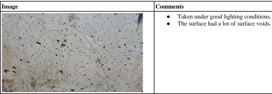
[image:2.595.72.515.569.723.2]Photographs of exposed concrete surfaces were taken from the ADD Building of the University of Nairobi. The Images were captured using a smartphone camera (Samsung Galaxy A7 (2017)). Each image had a resolution of 264×1836 pixels. Majority of the photos were taken under good lighting conditions in an afternoon.
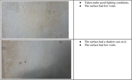
Table 1: Examples of photos collected
Image Comments
● Taken under good lighting conditions.
http://dx.doi.org/10.29322/IJSRP.9.06.2019.p9060 www.ijsrp.org
● Taken under good lighting conditions.
● The surface had few voids.
● The surface had a shadow cast on it.
● The surface had few voids.
Image Preprocessing and Dataset Creation
Preprocessing
Some of the raw photos were cropped into smaller 32×32 pixel images while the rest were cropped into 128x128 pixel images.
This was done so that both the small and large void could be adequately captured. Cropping was done using the Pillow1 and the
[image:3.595.70.524.54.331.2]sliding window technique. To make the process of cropping faster, the native python multiprocessing library was used.
Fig 1: Sliding Window technique
Source: Author
The sliding window technique is illustrated in Fig 1. Whenever the window slid to a new position, that portion of the image covered by the window was cropped and saved as an image file. The 32x32 images were obtained by using a 32x32 sliding window size, while the 128x128 images were obtained using a 128x128 sliding window size. Cropping was done on all the images until a databank of cropped images was produced.
Dataset Creation
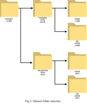
From the databank of cropped images, 2,016 images, showing voids, were chosen while an equal number of images, showing no voids, were also chosen. These two datasets were further split into training and validation datasets. The training data had a total of
http://dx.doi.org/10.29322/IJSRP.9.06.2019.p9060 www.ijsrp.org 3,218 images while the validation data had a total of 814 images. The data were arranged in a folder structure that is summarised in Fig 2.
Fig 2: Dataset folder structure
http://dx.doi.org/10.29322/IJSRP.9.06.2019.p9060 www.ijsrp.org Architecture and Parameters of the Model
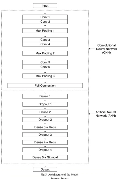
[image:5.595.92.496.86.703.2]Architecture
Fig 3: Architecture of the Model
Source: Author
Model Parameters
Table 2: Model Parameters
http://dx.doi.org/10.29322/IJSRP.9.06.2019.p9060 www.ijsrp.org
Input 32 32 Convolution 3 3 64 1
2 29 29 Convolution 2 2 64 1
3 14 14 Max Pooling 2 2 - 1
4 12 12 Convolution 2 2 128 1
5 11 11 Convolution 2 2 128 1
6 5 5 Max Pooling 2 2 - 1
7 4 4 Convolution 2 2 256 1
8 3 3 Convolution 2 2 256 1
9 1 1 Max Pooling 2 2 - 1
10 Full Connection
11 Dense 2048
12 Dropout 0.5
13 Dense 1024
14 Dropout 0.2
15 Dense 512
16 ReLu
17 Dropout 0.2
18 Dense 256
19 ReLu
20 Dropout 0.4
21 Dense 1
12 Sigmoid
Fig 3, represents the architecture with which the model was created. The model takes in an image of 32×32×3 pixel resolution. Each dimension indicates the height, width and colour channel respectively. The image passes through 3 convolutional layers, 6 ReLu(Nair and Hinton, 2010) layers, and 3 max pooling layers before being fully connected to the artificial neural network. The ANN consists of 5 Dense layers, 2 ReLu functions, 4 dropout layers and a Sigmoid function for classification.
Model Hyperparameters
The dropout rate for the dropout layers 17 and 20 are 0.2 and 0.4. The model made use of the binary cross entropy loss function which was optimised using mini-batch gradient descent. The gradient descent optimisation algorithm that was chosen was Adam
(Kingma and Ba, 2014) whose hyperparameters were a learning rate (⍺) of 0.001, β1of 0.9, β2of 0.999 and an epsilon (ε) of 1e
-07. Also, a batch size of 64 was used.
Workstation
Preprocessing and training were done on a workstation of the following specification: CPU: Intel i7-700HQ
RAM: 16GB
GPU: Nvidia GTX 1060 6GB VRAM
Training and validation
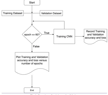
http://dx.doi.org/10.29322/IJSRP.9.06.2019.p9060 www.ijsrp.org Fig 4: Overview of training and validation
Source: Author
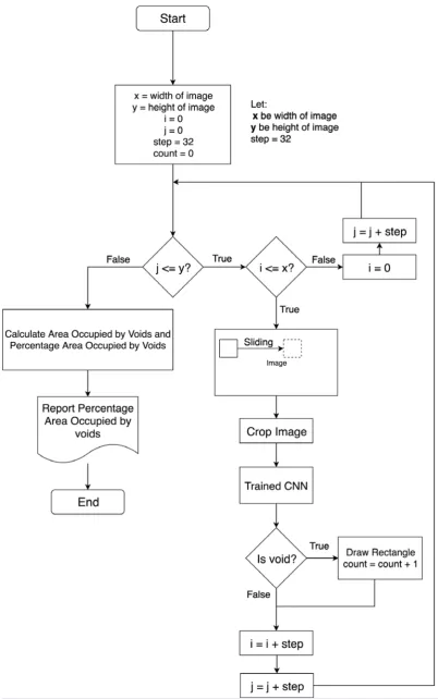
Creation of the Detector
The trained CNN was used to create a detector that could traverse an image larger than 32x32. This was implemented using Pillow, sliding window and the trained CNN. When the window slid to a new location, it cropped that part of the image,
converted it to a NumPy2 array, and then passed it to the CNN for prediction. When the prediction came by negative for a void,
the window slid to the next position. When the prediction came back positive for a void, the detector drew a rectangle around the perimeter of the sliding window before the sliding window moved to the next location.
2
http://dx.doi.org/10.29322/IJSRP.9.06.2019.p9060 www.ijsrp.org Fig 5: Overview of Detector
http://dx.doi.org/10.29322/IJSRP.9.06.2019.p9060 www.ijsrp.org Testing the Model
5 images from two different structures were taken with the aim of access the performance of the detector. 2 images were of a footbridge across University Way near the University of Nairobi main campus, which had a surface riddled with voids. The other 3 images were of a wall, near the American wing of the University of Nairobi, main campus, whose surface was visually intact.
Fig 6: Example of photo collected from the footbridge across University Way near the University of Nairobi main campus
Source: Author
Fig 7: Example of photo collected from the wall of a building near American Wing of the University of Nairobi, main campus
Source: Author
[image:9.595.37.231.517.702.2]3 additional photos of the surface of concrete cubes were taken from the concrete laboratory. The concrete was of a porous concrete mix.
Fig 8: Example of a photo of a cube made with a porous concrete mix
Source: Author
These images were used to perform 3 tests:
1. An image from the footbridge was used to determine the effect of varying the size of the sliding window on the detection
http://dx.doi.org/10.29322/IJSRP.9.06.2019.p9060 www.ijsrp.org
2. The images from the footbridge and the wall were used to gauge the accuracy of the CNN at detecting the voids.
3. The results from the images of the cubes were used to check whether there was a relationship between the percentage
area occupied by voids and actual porosity.
Results and Discussion
Testing and Validation Results
[image:10.595.100.505.262.477.2]During training, it took the model up to the 50th epoch to consistently hit a training accuracy of 90% and above. Before that, it would hit 90% accuracy sporadically with the first one occurring at the 38th epoch. The validation accuracy hit 80% accuracy as early as the 3rd epoch but would randomly fluctuate between the high-70s and mid-80s most of the time. The highest training accuracy obtained was 92.08% during the 58th epoch while the highest validation accuracy was 89.08% during the 46th epoch. This training and validation accuracies were adequate to provide a good foundation to build a performant void detector.
Fig 9: Accuracy Against Number of Epochs
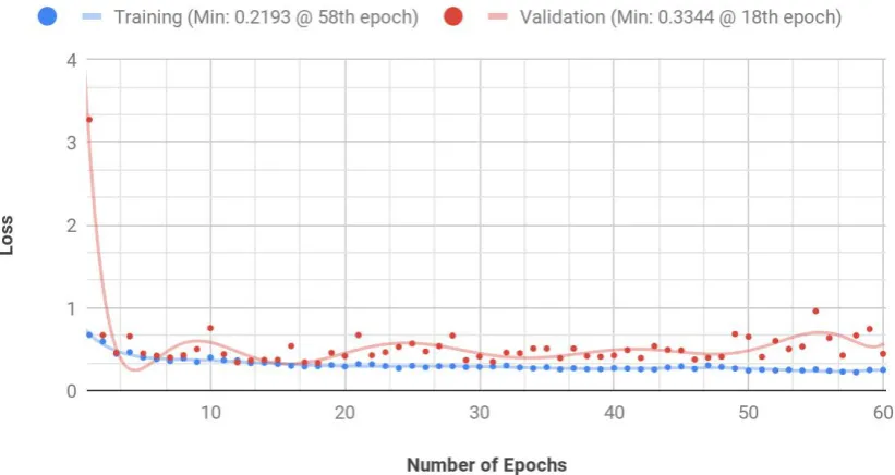
http://dx.doi.org/10.29322/IJSRP.9.06.2019.p9060 www.ijsrp.org Fig 10: Loss Against Number of Epochs
Finally, it can be seen from Table 3 that the best time to have stopped training was during the 12th epoch. This is because:
1. it had at a low validation loss of 0.3408 compared to the lowest of 0.3344 during the 18th epoch.
2. It had a high validation accuracy of 87.61% compared to the highest of 89.08% during the 46th epoch.
[image:11.595.172.424.429.631.2]Therefore, stopping should have been done early.
Table 3: Best Epochs to Stop Training
Epoch Val Accuracy (%) Val Loss
12 87.61 0.3408
13 84.91 0.3627
14 86.01 0.3706
15 85.52 0.3711
17 87.12 0.3413
18 86.99 0.3344
29 85.52 0.3666
31 87.48 0.3469
46 89.08 0.3758
Effect of Varying the Size of the Sliding Window
Table 4: Results of Varying Window Sizes
http://dx.doi.org/10.29322/IJSRP.9.06.2019.p9060 www.ijsrp.org 128x128
64x64
32x32
It was found that the largest window size (128x128) was best for detecting large voids. However, it could not adequately detect small voids. The smallest window size (32x32) performed the best at detecting small voids, but could not adequately detect large voids. Only the edges of the larger voids could be detected by the 32x32 window size.
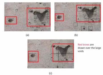
As it can be see from Fig 11, the 32x32 window size (a) performs the worst. The 64x64 (b) does a bit better. However, the best
http://dx.doi.org/10.29322/IJSRP.9.06.2019.p9060 www.ijsrp.org Fig 11: Detection of large voids: (a) 32x32 window, (b) 64x64 window and (c) 128x128 window
[image:13.595.116.479.60.323.2]It can be seen from Fig 11 that the detection of large voids increases with increase in window size.
Fig 12: Detection of small voids: (a) 32x32 window, (b) 64x64 window and (c) 128x128 window.
It can be seen from Fig 12 that the detection of small voids degrades with an increase in the window size. Furthermore, it can be seen that a 32x32 rectangle more closely wraps around the void compared to the larger rectangles. Therefore, a 32x32 window is better suited to calculate an estimate of the area occupied by voids.
Estimation of the Percentage Area Occupied by Voids
http://dx.doi.org/10.29322/IJSRP.9.06.2019.p9060 www.ijsrp.org 𝑟𝑎𝑡𝑖𝑜(%) =𝐴𝑟𝑒𝑎𝑇𝑜𝑡𝑎𝑙𝑜𝑐𝑐𝑢𝑝𝑖𝑒𝑑𝐴𝑟𝑒𝑎𝑜𝑓𝑏𝑦𝑃ℎ𝑜𝑡𝑜𝑣𝑜𝑖𝑑𝑠× 100
Table 5: Results of Estimating Percentage Area Covered by Voids
# Photo Area covered by voids
(%)
1 10.68%
2 49.62%
http://dx.doi.org/10.29322/IJSRP.9.06.2019.p9060 www.ijsrp.org
4 50.17%
5 6.64%
As expected the 32x32 window size could not adequately detect large voids present in photo 1 in Table 5. This could be because the small size doesn't give the model adequate information to make an accurate prediction when the sliding window is traversing a large void. However, photo 1 gave the best estimate of the area occupied by the voids compared to the other 4 photos. This could be because it had no stains (as seen in photo 2), no coarse surface (as seen in photos 3, 4 and 5) and had good lighting.
[image:15.595.71.524.54.407.2]
Fig 13: Model could not Detect Large Void When Using a 32x32 Sliding Window
http://dx.doi.org/10.29322/IJSRP.9.06.2019.p9060 www.ijsrp.org Fig 14: Accurate Prediction by the Model from Photo 2 of Table 5
[image:16.595.35.225.236.405.2]Secondly, the presence of stains in photo 2, cause the model to make a lot of false positive predictions hence giving inaccurate results. This is because the model was not trained on stained surfaces. Although the model was not trained on stained surfaces, the photo was chosen regardless in order to assess the performance of the model.
Fig 15: Stains on Concrete Surface Detected as Voids
Lastly, photo 3, 4 and 5 had a coarse finish to the surface. This coarseness was detected as void by the model even though the surfaces did not have any visible voids on them. This observation is elaborated below.
Effect of a Coarse Surface on Detection
When the detector comes across a coarse surface with no visible voids, the model detected that voids were present. This resulted in a lot of false-positives. This could be because the images that the model was trained on were of concrete surfaces that had a relatively smooth finish. The coarser surfaces on some of the test images, from the wall near the American Wing building, were not encountered during training.
[image:16.595.36.372.560.707.2]http://dx.doi.org/10.29322/IJSRP.9.06.2019.p9060 www.ijsrp.org Fig 17: Example of Coarse Surface
This behaviour of the model does introduce additional inaccuracies in results for Table 5.
[image:17.595.33.489.325.749.2]Detection of Voids on Surface of Porous Concrete
Table 6: Results of the detector on the surface of porous concrete
# 32x32 64x64 128x128
1
2
3
http://dx.doi.org/10.29322/IJSRP.9.06.2019.p9060 www.ijsrp.org
Sample 1 2 3
Window
Size 32 64 128 32 64 128 32 64 128
[image:18.595.34.495.54.122.2]Ratio (%) 6.13 11.04 28.27 26.91 35.39 65.27 4.45 14.09 31.88
Table 8: Actual Porosity Determined in the Laboratory
Sample Actual Porosity
1 23.6
2 24.5
[image:18.595.30.413.283.380.2]3 22.8
Table 9: Actual porosity and ratios obtained using different window sizes
Sample Actual Porosity
Ratio (% area occupied by voids)
32 64 128
1 23.6 6.13 11.04 28.27
2 24.5 26.91 35.39 65.27
3 22.8 4.45 14.09 31.88
Fig 18: Comparing Actual Porosity and Estimated Area occupied by Voids
[image:18.595.52.478.463.662.2]http://dx.doi.org/10.29322/IJSRP.9.06.2019.p9060 www.ijsrp.org Secondly, it can be observed that the size of the majority of the voids on the surfaces of the samples is large, hence it is not surprising that the 32x32 window size isn't adequate at detecting them. 64x64 and 128x128 performed much better with this regard. However, when 64x64 and 128x128 are compared, the 64x64 window size performed comparatively much better in certain situations. This is illustrated in Fig 19.
Fig 19: Performance of detector on photo 3 of Table 6: (a) 32x32 window, (b) 64x64 window, and (c) 128x128 window
Overall, as shown in Fig 18, the relationship between the percentage area covered by voids and actual porosity was unclear.
Problems With The Detector
1. The rectangles that the detector drew over the voids did not perfectly cover the voids.
Fig 20: (a) Rectangles don't perfectly cover voids and (b) Example of how rectangles should cover voids.
[image:19.595.53.304.527.711.2]http://dx.doi.org/10.29322/IJSRP.9.06.2019.p9060 www.ijsrp.org void while leaving the rest uncovered. This can be seen in Fig 20 (a) where
the top part isn’t covered. This resulted in an erroneous estimate of the area of the void.
2. The detector cannot dynamically adapt the size of the rectangles to cater for voids of different sizes.
Fig 21: (a) The rectangles are of the same size and (b) Example of how the model should vary the rectangle size
In many instances, the fixed rectangle size was sometimes inadequate at covering the voids. At times the voids were smaller than the rectangle leading to the rectangle capturing large portions of the concrete surface that did not have voids. Consequently, this gave a larger estimate of the area of the void. At other times, the voids were larger than rectangles hence the detector could not detect the voids all at once. It, therefore, relied on creating building blocks of smaller rectangles in order to cover the voids entirely. This can be seen in Fig 14. However, if the voids were too large, the detector would fail to detect the parts of the voids that did not have edges in them. Therefore, the detector wouldn’t draw rectangles around those portions, consequently giving a lower estimate of the area of the void. This can be seen in Fig 13.
Conclusion and Recommendation
Conclusion
From this study, the following conclusions were made:
1. CNNs are an effective way of detecting voids. Accuracies of 92.08% and 89.08% were obtained during training and
validation respectively.
2. The larger the sliding window size, the more effective it is at detecting large voids. However, the larger the sliding
window size, the less effective it is at detecting small voids and vice versa.
3. The relationship between the percentage area covered by voids and actual porosity was unclear.
Recommendations
It is recommended that an established object detection algorithm such as region proposal techniques, YOLO and SSD be used. This is because they produce closely fitting bounding boxes compared with the simple sliding window algorithm used in this study. They can also produce bounding boxes of different sizes depending on the size of the object.
It is also recommended that more data be collected so that the CNN can be able to learn how to detect voids under different concrete surface conditions.
References
1. ACI Committee 301. (2010). Specifications for Structural Concrete: (ACI 301-10). Farmington Hills, MI: American
Concrete Institute
2. ACI Committee 347. (2004). Guide to formwork for concrete: (ACI 347-04). Detroit, Mich: American Concrete
Institute.
[image:20.595.63.475.134.282.2]http://dx.doi.org/10.29322/IJSRP.9.06.2019.p9060 www.ijsrp.org
4. Cha, Y.J., Choi, W. and Büyüköztürk, O., (2017). “Deep learning‐based crack damage detection using convolutional
neural networks”, Computer‐Aided Civil and Infrastructure Engineering, 32(5), pp.361-378.
5. Girshick, R., (2015). Fast r-cnn. In Proceedings of the IEEE international conference on computer vision (pp.
1440-1448).
6. Girshick, R., Donahue, J., Darrell, T. and Malik, J., (2014). Rich feature hierarchies for accurate object detection and
semantic segmentation. In Proceedings of the IEEE conference on computer vision and pattern recognition (pp. 580-587).
7. Iffat, S., (2015). “Relation between density and compressive strength of hardened concrete”, Concrete Research Letters,
6(4), pp.182-189.
8. Kingma, D.P. and Ba, J., (2014). Adam: A method for stochastic optimization. arXiv preprint arXiv:1412.6980.
9. Krizhevsky, A., Sutskever, I. and Hinton, G.E., (2012). “Imagenet classification with deep convolutional neural
networks”. Advances in neural information processing systems, (pp. 1097-1105)
10. Liu, W., Anguelov, D., Erhan, D., Szegedy, C., Reed, S., Fu, C.Y. and Berg, A.C., (2016). “SSD: Single shot multibox
detector”. In European conference on computer vision (pp. 21-37). Springer, Cham.
11. Nair, V. and Hinton, G.E., (2010). Rectified linear units improve restricted boltzmann machines. In Proceedings of the
27th international conference on machine learning (ICML-10) (pp. 807-814).
12. Redmon, J., Divvala, S., Girshick, R. and Farhadi, A., (2016). “You only look once: Unified, real-time object detection”.
In Proceedings of the IEEE conference on computer vision and pattern recognition (pp. 779-788).
13. Ren, S., He, K., Girshick, R. and Sun, J., (2015). Faster r-cnn: Towards real-time object detection with region proposal
networks. In Advances in neural information processing systems (pp. 91-99).
14. Teidj, S., Khamlichi, A. and Driouach, A., (2016). “Identification of beam cracks by solution of an inverse problem”.
Procedia Technology, 22, pp.86-93.
15. Xu, L. and Huang, Y. (2017). “Effects of Voids on Concrete Tensile Fracturing: A Mesoscale Study”. Advances in
Materials Science and Engineering, 2017, pp.1-14.
16. Yokoyama, S. and Matsumoto, T., (2017). Development of an automatic detector of cracks in concrete using machine
learning. Procedia engineering, 171, pp.1250-1255.
17. Ziou, D. and Tabbone, S., (1998). “Edge detection techniques-an overview”. Pattern Recognition and Image Analysis