http://dx.doi.org/10.4236/jmf.2016.61016
Statistical Arbitrage in S&P500
Stefanos Drakos
International Centre for Computational Engineering, Rhodes, Greece
Received 8 January 2016; accepted 24 February 2016; published 29 February 2016
Copyright © 2016 by author and Scientific Research Publishing Inc.
This work is licensed under the Creative Commons Attribution International License (CC BY).
http://creativecommons.org/licenses/by/4.0/
Abstract
A methodology to create statistical arbitrage in stock Index S&P500 is presented. A synthetic asset based on the cointegration relationship of the stocks with Index was constructed. In order to cap-ture the dynamic of the market time adaptive algorithms have been developed and discussed. The pair trading strategy was applied in different periods between S&P500 and synthetic asset and the results were evaluated. Different metrics have shown that the Multvariate Kalman Algorithm creates statistical arbitrage in index with much lower Maximum Drawdown and higher profit. The algorithm is neutral as the beta is close to zero and the Sharp Ratio remains high in all cases.
Keywords
Statistical Arbitrage, Mean Reverting, Pair Trading, Kalman Filter, Trading Algorithms
1. Introduction
Financial markets are based on the general trading rule: buy with low price and sell with high price. The aim is the development of strategies with low risk and succeeds this general rule. Pure Arbitrage is a category of strat-egies with zero risk. As an example we can refer the case of buying and selling a stock at the same time with a different value in two different exchanges. The profit results from the difference in prices, breaking the law of one price.
the idea that two assets with the same features can be priced about the same price as the basis of the law of one price. When at a given time the stock prices are different then one is overvalued and the other undervalued rela-tive to the actual price. The classic trading Pairs strategy derives from the characteristics of this incorrect pricing (mispricing) between the two stocks.
In the current work instead of the two stocks the mispricing between the index S&P500 and a sub-set of stocks belonging to this is considered. This forms a portfolio consisting of one unit of the Index in long (or short) and the corresponding number γ (Hedge ratio) of subset’s stocks in the opposite position. Three methods adopted to determine the number γ (Hedge ratio): a) the ordinary, b) the rolling ordinary least squares (OLS) re-gression and c) the Kalman filter process as it is presented below. According to the strategy, the spread of the index S&P500 and the stocks prices’ combination are computed and when this deviates from its historical aver-age value then the investor bets on the return to the historical with selling and buying respectively the stocks of the portfolio. In practice to construct the synthetic asset is necessary to investigate the appropriate stock exhibit-ing long relationship between them with the index. The technique used for this purpose is the Cointegration as this presented in [1] according to which two time series Xt ~I
( )
1 and Yt ~I( )
1 are cointegrated if( )
~ 0
t t
aX +bY I for a b, ≠0 and notation I(d) means integrated order d.
In [1] concluded that pairs who cointegrate in sample period behave better in the out-of-sample period than those not cointegrate in the sample period. Based on the previous, the spread of the linear combination of the cointegrated stocks and the S&P500 index have to be stationary process. To analyze this relationship the aug-mented Dickey-Fuller test (ADF) was used as presented in [2]. According to the strategy the stocks are not re-stricted to cointegrate in the out-of-sample period but it is an indication that they will present mean-reverting behavior.
Additionally the log of prices used is also instead the prices as in [3]. The main reason is that log-returns are time additive. So, in order to calculate the return over n periods using real returns we need to calculate the prod-uct of n numbers:
(
1+r1)(
1+r2) (
1+rn)
.If r1 defined as:
(
)
1 0 1
1 1
0 0
1
P P P
r r
P P
−
= ⇒ + = (1)
And
(
)
11
0
log 1 r log P P
+ =
(2)
(
)
(
)
(
)
( )
( )
( )
( )
( )
(
)
( )
( )
1 2
1 2
0 1 1
1 0 2 1 1
0
log 1 log 1 log 1
log log log
log log log log log log
log log n n n n n n
r r r
P
P P
P P P
P P P P P P
P P − − + + + + + + = + + + = − + − + + − = −
Consequently the profit of spread over a period is equal to:
log log
A
t i t i
t i t A
t t
P P
y y
P γ P
Β
+ +
+ Β
− = −
(3)
2. Period of Methodology
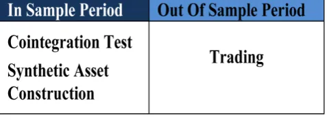
The proposed methodology and the trading algorithm designed based on that divided in two different spaces. The first refers to the in sample period which is used to make all the appropriate test and construct the synthetic asset and the other to the out of sample period (Trading Period) where the synthetic asset trading based on the specific rules (Figure 1).
2.1. In Sample Period
The data of the in sample period used for the synthetic asset construction. Working on a daily data domain a year of closing prices was chosen as the in sample period for determine the set of cointegrated stocks with S&P500 and create the synthetic asset.
Synthetic Asset Construction.
The paper presents different algorithms in order to create statistical arbitrage in S&P500. The S&P500, based on the market capitalizations of 500 large companies equity indices, and many consider it one of the best represen-tations of the U.S. stock market. The initial choice of stocks for cointegration test with S&P500 is made by the S&P100 which is a sub-set of the S&P500, and measures the performance of large cap companies in the United States. Constituents of the S&P100 are selected for sector balance and represent about 57% of the market capita-lization of the S&P500 and almost 45% of the market capitacapita-lization of the U.S. equity markets. The stocks in the S&P100 tend to be the largest and most established companies in the S&P500 (Wikipedia).
Using the data of a selected In Sample Period for each stock Si∈S&P 100 the second step of Engle and Granger’ approach adopted. Using the logarithmic price of stocks and S&P500 the OLS regression shown below is performed:
( )
( )
log StSPY =
γ
ilog Sti +ε
t (4)Τhe Augmented Dickey-Fuller unit root test applied for the stationarity of the OLS residuals. According to the successful stationary result a subset of the S&P100 is created and the components of this set are the candidate for the synthetic asset construction. Still working in the sample period a new OLS regression was carried out:
(
)
( )
log SPY Nlog i
t i t t
S =γ
∑
S +ε (5)Or
(
)
(
)
log SPY log N i
t i t t
S =γ
∏
S +ε (6)Using again the Augmented Dickey-Fuller the stationarity of the new OLS residuals is examined.
If the stationarity exist then this an evidence of mean reverting long term behavior of the spread
(
)
( )
log SPY Nlog i
t St i St
ε = −γ
∑
where Sti∈S and S is the set of stock where individually and as logarithmic sum cointegrated with S&P500. The dimension of S is dim(S).2.2. Out of Sample Period-Trading Period
[image:3.595.196.435.617.705.2]According to the previous period different algorithms for synthetic asset trading are developed. The first was
designed assumed that the cointegration coefficient is constant during the trading period.
In that case and using the Equation (3) the profit of the strategy during the period t ÷ t + h arises from the fol-lowing equation:
log log
SPY i
N
t h t h
t h t SPY i i
t t
S S
S S
ε ε + γ +
+
− = −
∑
(7)3. Time Adaptive Coefficient
γ
In reality the system of trading is dynamic and updated as new information get to in and the cointegration coefe-cient (or the hedge ratio) cannot stay constant during the trading period. For that reason time adaptive algorithms are developed to capture the real conditions of the markets.
3.1. Rolling Ordinary Least Squares (OLS) Regression
The first one considering a rolling ordinary least squares (OLS) regression. The frequency of regression calcula-tions raised by an optimization procedure and the cointegration coefficient calculated at each step by the regres-
sion of log
( )
SPY tS against the log
(
N i)
t i S∏
.3.2. Kalman Filter Process
The Kalman filter process can be described by three different steps: the prediction the observation and the cor-rection. A new approach were developed using a Multivariate Kalman filter process. Based on that the hedge ra-tio calculated separately for each stock owned in the synthetic asset and the computed vector of the calculated parameters at each time step has dimensions (N + 1) × 1 where N = dim(S) while the dimensions of the cova-riance matrix is (N + 1) × (N + 1). The aim of these algorithms is to calculate at each time step the updated hedge ratio of the synthetic asset. Assuming that the hedge ratio and the premium follow a random walk we have:
1
t t t
y =y− +w (8) where:
yt: is the current state of the of the parameters.
yt-1: is the previous state of the of the parameters.
(
)
~ 0,
t w
w N
σ
where for the multivariate Kalman filter process
T
1 2 n
t t t t t
y = γ γ γ µ (9)
With:
[
]
T0 0
y = h h h
µ
(10) h: is the cointegration coefficient from in sample period and μ0 coming from the same period.The vector of logarithmic price of stocks:
( )
1( )
2( )
log log log n 1
t t t t
x = S S S (11)
And Sti∈S
The process following the steps as below:
Prediction state where the next system state is predicted based on the knowledge of the previous state
| 1 | 1 ˆt t t t t
y − = y − +w (12) The covariance of prediction state is given by:
| 1 1| 1
ˆ ˆ
t t t t w
P − =P− − +V (13)
hedge ratio the measurement prediction are given as:
| 1
ˆ ˆt t t t
z = ⋅x y − (14)
The residual of measurement and real value at each step calculated as:
( )
ˆlog SPY
t St zt
ε
= − (15)The variance of measurement error is equal to:
T | 1
ˆ
t t t t t e
S =x P⋅ − ⋅x +V (16)
The Kalman Gain is the filter, which tells how much the predictions should be corrected on time step is given as:
T | 1
ˆ t t t t t P x K S − ⋅
= (17)
The last step of process is the update step where: The updated state is estimated as following:
| | 1
ˆt t ˆt t t t
y = y − +K ⋅ε (18)
And the Updated state covariance is equal to
| | 1
ˆ ˆ T
t t t t t t t
P =P − −K ⋅ ⋅S K (19)
All the process repeated at every time step of out of sample period. The estimation of Vw and Ve has been
dis-cussed in [11] [12].
3.3. Profit of Strategies
In the case of Time Adaptive coefficient γ of the linear regression case the profit of the pair trading strategy raised by the following equations:
log log t h t N i SPY t h i t h
t h t SPY N
i t t i S S S S γ γ ε ε + + + + − = −
∏
∏
(20)In the case of Multivariate Kalman Filter where the hedge ratio is different for each stock and for each time step in the synthetic asset it can been shown that:
(
)
(
( )
( )
( )
)
(
)
11 1 2 2
1 1 1 1 1 1 1 1
1 1
log log log log
log log i
SPY n n
N
SPY i
i
S S S S
S γ S
ε = − γ +γ + +γ
= −
∏
Similarly( )
( )
22 2 2
h h log log log log i i t h N SPY i i N SPY i
t t t h
i S S S S γ γ ε ε + + + + = − = −
∏
∏
And finally the profit during a period t t+h is equal to:
log log i t h i t N i SPY t h
t h i
t h t SPY N i
t t i S S S S γ γ
ε ε + + +
+ − = −
∏
4. The Pair Trading Strategy
The algorithm of the pair trading strategy is based on the distance of the spread from its historical mean value and its mean-reverting behavior. To measure this distance a normalized variable called z-score introduced as:
[ ]
( )
t t
t
t
z ε ε
σ ε
−
= (22)
where:
[ ]
ε
t : is the mean value of the spread over a lookback period.
( )
tσ ε
: is the standard deviation of the spread over the same period.The trading it takes place when this variable exceeds some limits based on the spread mean reverting behavior. Thus:
Open-long position if zt<zlow. Open-short position if zt >zhigh. Exit-long position if zt>zexit-low. Exit-short position if zt <zexit-high.
When a long (short) position is opened we buy (sell) one unit of S&P500 and sell (buy) the following amount
of stocks from synthetic asset as: Nlog
( )
i ti S
γ
∑
in the case of constant hedge ratio, Nlog( )
it i St
γ
∑
when therolling OLS regression is applied, and
∑
iNγtilog( )
Sti if the Kalman Filter algorithm applied. The performance of strategy evaluated using the following metrics: 1) Cumulative return, 2) Annualized Return, 3) Sharpe Ratio, 4) Maximum drawdown, 5) beta.5. Back Testing-Performance Evaluation
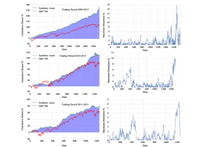
Five different time periods was studied. In each case one year data collection was used in order to make the en-tire test and construct the synthetic asset. After that the algorithm starts trading with ending day for all cases the 30/12/2015. All the sample periods started at the first day of the year and ending at the last of the same year. The trading started on the first day the next year. In Table 1 the back testing periods are presented. In Figure 2 and
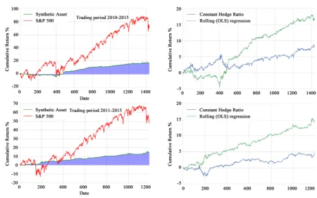
Figure 3 the results of cumulative return of Multivariate Kalman Filter algorithm against S&P500 and its max-imum drawdown are shown. In Figure 4 and Figure 5 the cumulative return of rolling OLS regression algo-rithm against S&P500 and the cumulative return of rolling OLS regression algoalgo-rithm against constant hedge ra-tio are illustrated. In t Table 2 the sets of synthetic assets are presented while in Table 3 the name of symbols is given. In Tables 4-8 all the metrics of the algorithms are displayed.
It can be shown that the dimension of the set and the constituents are different from period to period. This is an evidence of the non constant cointegration behavior of the stocks with the index but as we can see from the graphs the synthetic asset of each period continues to trade with profit and good metrics results.
Table 1. Back testing periods.
2006 2007 2008 2009 2010 2011 2012 2013 2014 2015
In Sample Trading
2007 2008 2009 2010 2011 2012 2013 2014 2015
In Sample Trading
2008 2009 2010 2011 2012 2013 2014 2015
In Sample Trading
2009 2010 2011 2012 2013 2014 2015
In Sample Trading
2010 2011 2012 2013 2014 2015
Table 2. Sets of stock in synthetic asset on each period.
Trading Period Stock of Synthetic Asset (Set S) Dim (S)
2007-2015 {BRK.B, DVN, IBM, SPG} 4
2008-2015 {CAN, BAX, BMY, DELL, EMC, GE, HAL, MDLZ, NSC, T, TXN, VZ} 12
2009-2015 {DVN, FCX, IBM, MON, SPG} 5
20010-2015 {APA, AXP, C, CAT, COF, FCX, IBM, MMM} 8
[image:7.595.106.533.241.496.2]2011-2015 {COST, FDX, GS, QCOM} 4
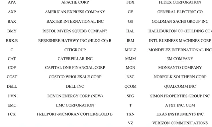
Table 3. Union set of companies raised from cointegration test from all the period of study.
APA APACHE CORP FDX FEDEX CORPORATION
AXP AMERICAN EXPRESS COMPANY GE GENERAL ELECTRIC CO
BAX BAXTER INTERNATIONAL INC GS GOLDMAN SACHS GROUP INC
BMY RISTOL MYERS SQUIBB COMPANY HAL HALLIBURTON CO (HOLDING CO)
BRK.B BERKSHIRE HATHWY INC (HLDG CO) B IBM INTL BUSINESS MACHINES CORP
C CITIGROUP MDLZ MONDELEZ INTERNATIONAL INC
CAT CATERPILLAR INC MMM 3M COMPANY
COF CAPITAL ONE FINANCIAL CORP MON MONSANTO COMPANY
COST COSTCO WHOLESALE CORP NSC NORFOLK SOUTHERN CORP
DELL DELL INC QCOM QUALCOMM INC
DVN DEVON ENERGY CORP (NEW) SPG SIMON PROPERTIES GROUP INC
EMC EMC CORPORATION T AT&T INC. COM
FCX FREEPORT-MCMORAN COPPER&GOLD B TXN EXAS INSTRUMENTS INC
[image:7.595.92.538.522.720.2]VZ VERIZON COMMUNICATIONS
Table 4. Statistical metrics performance for the trading period 01/01/2007-30/12/2015. In Sample Period 01/01/2006-31/12/2006
S&P500
Out of Sample Period 01/01/2007-30/12/2015
Algorithm
MultiVariate Kalman Filter Rolling (OLS) regression Constant Hedge Ratio
Cumulative Return % 387.069 24.637 12.678 45.592
Annual Return % 19.261 2.481 1.337 4.268
Sharpe Ratio 3.298 0.892 0.483 0.303
Beta 0.019 0.017 0.027
Maximum Drawdown % 12.642 2.925 5.666 62.453
Duration of Maximum
Table 5. Statistical metrics performance for the trading period 01/01/2008-30/12/2015 In Sample Period 01/01/2007-31/12/2007
Out of Sample Period 01/01/2008-30/12/2015
Algorithm
Multi Variate Kalman Filter Rolling (OLS)
regression Constant Hedge Ratio S&P500 Cumulative Return % 171.671 22.347 6.855 42.470
Annual Return % 13.321 2.556 0.833 4.528
Sharpe Ratio 1.135 0.738 0.228 0.312
Beta −0.010 −0.005 −0.013
Maximum Drawdown % 28.636 6.730 5.301 52.909
Duration of Maximum
Drawdown 175.0 404.0 628.0 154.0
Table 6. Statistical metrics performance for the trading period 01/01/2010-30/12/2015 In Sample Period 01/01/2008-31/12/2008
S&P500
Out of Sample Period 01/01/2009-30/12/2015
Algorithm
MultiVariate Kalman Filter Rolling (OLS)
regression Constant Hedge Ratio
Cumulative Return % 278.267 28.513 13.565 121.512
Annual Return % 20.972 3.655 1.837 12.054
Sharpe Ratio 3.039 1.387 0.753 0.729
Beta 0.026 −0.003 0.032
Maximum Drawdown % 17.910 3.934 3.736 28.547
[image:8.595.96.537.533.721.2]Duration of Maximum Drawdown 69.000 290.000 367.000 203.0
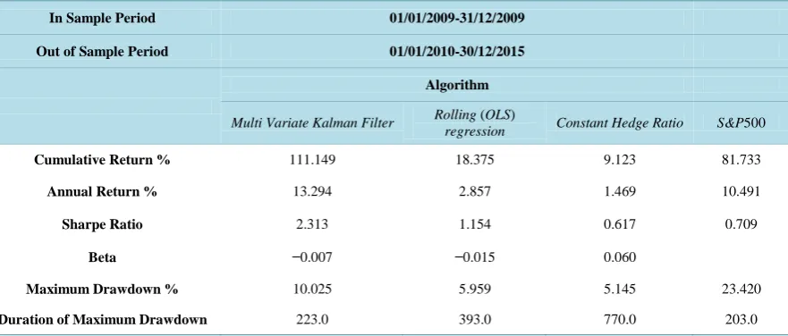
Table 7. Statistical metrics performance for the trading period 01/01/2010-30/12/2015 In Sample Period 01/01/2009-31/12/2009
Out of Sample Period 01/01/2010-30/12/2015
Algorithm
Multi Variate Kalman Filter Rolling (OLS)
regression Constant Hedge Ratio S&P500 Cumulative Return % 111.149 18.375 9.123 81.733
Annual Return % 13.294 2.857 1.469 10.491
Sharpe Ratio 2.313 1.154 0.617 0.709
Beta −0.007 −0.015 0.060
Maximum Drawdown % 10.025 5.959 5.145 23.420
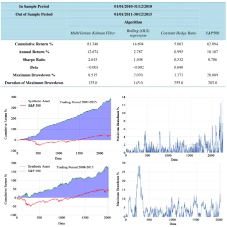
Table 8. Statistical metrics performance for the trading period 01/01/2011-30/12/2015 In Sample Period 01/01/2010-31/12/2010
Out of Sample Period 01/01/2011-30/12/2015
Algorithm
MultiVariate Kalman Filter Rolling (OLS)
regression Constant Hedge Ratio S&P500 Cumulative Return % 81.346 14.694 5.063 62.094
Annual Return % 12.674 2.787 0.995 10.167
Sharpe Ratio 2.643 1.408 0.532 0.706
Beta −0.003 −0.002 0.040
Maximum Drawdown % 8.515 2.070 3.373 20.889
Duration of Maximum Drawdown 125.0 143.0 255.0 203.0
Figure 2. Cumulative return and drawdown diagram for multivariate kalman filter algorithm for the trading periods starting
at 2007, 2008 and ending at 2015. Comparing the metrics of each period of study it is clear the Multivariate Kalman Filter algorithm gives the
Figure 3. Cumulative return and drawdown diagram for multivariate kalman filter algorithm for the trading periods starting
at 2009, 2010, 2011 and ending at 2015.
Figure 4. Cumulative return of rolling ols regression algorithm against S&P500 and algorithm with constant hedge ratio, for
[image:10.595.157.473.412.694.2]Figure 5. Cumulative return of rolling OLS regression algorithm against S&P500 and algorithm with constant hedge ratio,
for trading period starting at 2010, 2011 and ending at 2015. with higher MDD = 23.42 and duration = 203. The SR of MKFA is still higher and equal to 2.313. In the last
periods the profits declined but kept higher profit and Sharp Ratio than S&P500.
The second algorithm of rolling OLS regression gives lower cumulative profit than Index but has almost doubled Sharp Ratio than S&P500 in all cases. Finally the evaluation of metrics has shown that the MKFA can beat the market as it creates statistical arbitrage condition in Index.
6. Conclusion
Mean-reverting algorithms with time adaptive hedge ratio are presented. A methodology of a synthetic asset construction based on the stocks of S&P500 has been discussed. The criterion of the selection was the cointegra-tion relacointegra-tionship of individual stocks as the logarithmic sum of them with S&P500. The results of back testing show that for different period of study the form and the dimension of the synthetic asset are different. Pair trad-ing strategy was adopted and the evaluation of the metrics results presented better behavior of MKFA among the others and beat the market. In the last periods the profits declined but it was still higher than S&P500 with much higher Sharp Ratio. The algorithm defended better its profit as the Maximum Draw down was quite lower than Index.
References
[1] Engle, R. and Granger, C. (1987) Co-Integration and Error Correction: Representation, Estimation, and Testing. Eco-nometrica, 55, 251-276. http://dx.doi.org/10.2307/1913236
[2] Vidyamurthy, G. (2004) Pairs Trading, Quantitative Methods and Analysis.John Wiley & Sons, Hoboken.
[3] Infantino, L. and Itzhaki, S. (2010) Developing High-Frequency Equities Trading Models. Master of Business Admin-istration, Massachusetts Institute of Technology, Cambridge.
[4] Ernie, C. (2013) Algorithmic Trading: Winning Strategies and Their Rationale. John Wiley & Sons, Hoboken.
[6] Dunis, C.L. and Ho, R. (2005) Cointegration Portfolios of European Equities for Index Tracking and Market Neutral Strategies. Journal of Asset Management, 6, 33-52. http://dx.doi.org/10.1057/palgrave.jam.2240164
[7] Dunis, C.L, Giorgioni, G., Laws, J. and Rudy, J. (2010) Statistical Arbitrage and High-Frequency Data with an Appli-cation to Eurostoxx 50 Equities. CIBEF Working Papers, CIBEF.
[8] Elliott, R., van der Hoek, J. and Malcolm, W. (2005) Pairs Trading. Quantitative Finance, 5, 271-276. http://dx.doi.org/10.1080/14697680500149370
[9] Gatev, E., Goetzmann, W.N. and Rouwenhorst, K.G. (2006) Pairs Trading: Performance of a Relative-Value Arbitrage Rule. Review of Financial Studies, 19, 797-827. http://dx.doi.org/10.1093/rfs/hhj020
[10] Khandani, A. and Lo, A.W. (2007) What Happened to the Quants in August 2007. http://web.mit.edu/Alo/www/Papers/august07.pdf
[11] Rajamani, M. (2007) Data-Based Techniques to Improve State Estimation in Model Predictive Control.PhD Thesis, University of Wisconsin-Madison, Madison.