Modeling Long Memory in REITs

Munich Personal RePEc Archive

Modeling Long Memory in REITs

Cotter, John and Stevenson, Simon

2007

Online at

https://mpra.ub.uni-muenchen.de/3500/

Modeling Long Memory in REITs

John Cotter, University College Dublin

Centre for Financial Markets, School of Business, University College Dublin, Blackrock, County Dublin, Republic of Ireland. E-Mail: [email protected]

and

Simon Stevenson, Cass Business School, City University

Faculty of Finance, Cass Business School, City University, 106 Bunhill Row, London, EC1Y 8TZ, UK. Tel: +44-20-7040-5215, Fax: +44-20-7040-8881, E-Mail: [email protected]

Current Draft: May 2007

* _{Author to whom correspondence should be addressed. The authors would like to}

Modeling Long Memory in REITs

Abstract

One stylized feature of financial volatility impacting the modeling process is long

memory. This paper examines long memory for alternative risk measures, observed

absolute and squared returns for Daily REITs and compares the findings for a market

equity index. The paper utilizes a variety of tests for long memory finding evidence

that REIT volatility does display persistence. Trading volume is found to be strongly

associated with long memory. The results do however suggest differences in the

findings with regard to REITs in comparison to the broader equity sector.

Modeling Long Memory in REITs

1. Introduction

The continued development and increased investor awareness of the Real Estate

Investment Trusts (REIT) sector has led to a dramatic increase in daily trading in the

sector in recent years. SNL Financial estimate that average daily volume has increase

from just over 7m shares in 1996 to over 40m shares in 2005. In addition, as the sector

continues to mature and develop there will be is increased interest in derivative

products based on the sector. At present a number of OTC (over-the-counter) products

are available, while the Chicago Board Options Exchange (CBOE) provides traded

options on the Dow Jones Equity REIT Index. The growth in both traded and OTC

derivative products based on REITs furthers the interest in the dynamics of the sector

at higher frequencies such as daily intervals. Furthermore, an examination of the

volatility of the sector becomes more important as not only daily trading increases,

but also as a result of its role in derivative pricing.

In contrast to the large literature that has examined the return behavior of REITs, very

few examine volatility in the sector, and even fewer use high frequency data. Two

early papers on REIT volatility (Devaney, 2001 and Stevenson, 2002a) both analyzed

monthly data. The analysis conducted by Devaney (2001) was primarily concerned

with the sensitivity of REIT returns and volatility to interest rates and was undertaken

using a GARCH-M framework. The Stevenson (2002a) paper was, in contrast,

concerned with volatility spillovers across both different REIT sectors, and between

REITs and the equity and fixed-income markets. Four recent papers have examined

various aspects of daily REIT volatility. Winniford (2003) concentrates on seasonality

in REIT volatility. The author finds strong evidence that volatility in Equity REITs

varies on a seasonal basis, with observed increased volatility in April, June,

September, October and November. Cotter & Stevenson (2006) utilize a multivariate

GARCH model to analyze dynamics in REIT volatility. Using a relatively short and

quite distinct period of study (1999-2003) they find an increasing relationship

between Equity REITs and mainstream equities in terms of both returns and volatility.

Bredin et al. (2008), as with the Devaney (2001) paper, concentrate on the specific

Fed Funds Rate on REIT volatility. The results show a significant response in REIT

volatility to unanticipated rate changes, however in contrast to much of the broader

equity market evidence no evidence of asymmetry in the response in found. The final

paper to have examined daily REIT volatility is the one most similar to the current

paper. Najand & Lin (2004) utilize both GARCH and GARCH-M models in their

analysis, reporting that volatility shocks are persistent.

This persistence in volatility is a common empirical finding in financial economics

and is studied extensively in Taylor (1986). Whereas asset returns have largely been

found to contain very little autocorrelation, it has been noted in a large number of

papers across different asset classes that autocorrelation in various measures of

volatility does exist at significant levels and remains over a large number of lags1.

This effect, referred to as long memory, has been documented across a large sphere of

the finance literature from macroeconomic series such as GNP (Diebold &

Rudebusch, 1989) to exchange rate series (Baillie et al., 1996; Andersen & Bollerslev,

1997a, 1997b) at low and relatively high frequencies. Moreover, it is documented for

equity index series at daily intervals (Ding et al., 1993, Ding & Granger, 1996).

This paper examines the long memory properties of alternative risk measures,

observed absolute and squared returns for REITs and compares these to the S&P500

composite index. Analysis of long memory has been overlooked and we benchmark

our REIT findings against the broader equity market. Specifically, the long memory

property and its characteristics are explored. The long memory property occurs where

volatility persistence remains at large lags and the series are fractionally integrated.

Fractionally integrated series are integrated to order d where 0 < d < 1 unlike

integrated series of order 1, d = 1, and non-stationary series of order 0, d = 0.

Fractionally integrated series have observations far apart in time that may exhibit

weak but non-zero correlation. Much focus has been on the absolute returns

series,R_tk, or a squared returns series, [Rt2]k, for different power transformations,

k>0. This property adds to the general clustering condition usually referred to in the

context of squared returns persistence originally modeled in Engle’s (1982) ARCH

paper. There are daily cycles to the dependence structure giving rise to daily

involves a u-shaped cyclical pattern (Andersen & Bollerslev, 1997a, 1997b). In

addition, Ding et al. (1993) indicate that this non-linear dependence is strongest for

absolute volatility with a power transformation of k=1 and as a consequence they

suggest that parametric modeling of volatility should focus on absolute returns rather

than the commonly used squared returns.

This paper begins by examining the autocorrelation structure of the REIT returns and

volatility series. It then formally tests for the long memory property and measures the

magnitude of the fractional integration parameter. In terms of model building, there

are several approaches from linear and non-linear perspectives that could be applied.

This paper fits two long memory volatility models, Fractionally Integrated GARCH

(FIGARCH) and Fractionally Integrated Exponential GARCH (FIEGARCH) that

allow for asymmetry. Baillie et al. (1996) find that these models have considerable

success in modeling daily equity returns and we will investigate whether these

GARCH models can capture the long memory properties of daily REITS. The paper

examines the association between volume and volatility in the long memory volatility

models. The paper proceeds as follows. In Section 2, long memory is discussed. The

section incorporates a presentation and discussion of our GARCH models that are

fitted to the daily series’. Details of the series and data capture follow in Section 3.

Section 4 presents the empirical findings. It begins by briefly describing the indicative

statistics of the volatility series’, followed by a thorough analysis of their long

memory characteristics. In addition, the ability of the GARCH processes to model

volatility persistence is presented. Finally, a summary of the paper and some

conclusions are given in section 5.

2. Long Memory

Baillie (1996) shows that long memory processes have the attribute of having very

strong autocorrelation persistence before differencing, and thereby being

non-stationary, whereas the first differenced series does not demonstrate persistence and is

stationary. However, the long memory property of these price series is not evident

from just first differencing alone, but has resulted from analysis of the associated risk

measures. In fact financial returns themselves have only been found to exhibit short

subsequent lags. Thus the finance literature has concentrated its analysis of long

memory on the volatility series and we follow this convention.

Long memory properties may be investigated by focusing on the absolute returns

series denoted absolute volatility, R_t k, or the squared returns series denoted squared

volatility, [Rt2]k, and on their power transformations, where k>0.2 Absolute volatility

is examined as Davidian & Carroll (1987) find that absolute realizations are more

robust in the presence of fat-tailed observations found in financial series than their

squared counterparts. Moreover, empirical analysis of financial time series suggests

that the long memory feature dominate for absolute over squared realizations (see

Ding & Granger, 1996). Whereas squared volatility is utilized given that it underpins

the commonly used risk measures such as standard deviation and variance.

Models with a long memory property have dependency between observations of a

variable for a large number of lags so that Cov[Rt+h, Rt-j, j≥0] tends to zero as the

number of lags h gets large.3 In particular, long memory in financial time series has

concentrated on volatility realizations where unexpected shocks affect the series for a

large time frame. Thus confirmation of long memory properties for REITS would

have major implications for the associated investments strategies that need to take

account of the persistence and characteristics of the dependence structure in REIT

volatility. However, if the dependency between observations of a variable disappears

for a small number of lags, h, such as for a stationary ARMA process, then the data is

described as having a short memory property and Cov[Rt+h, Rt-j, j≥0] → 0. Formally,

long memory is defined for a weakly stationary process if its autocorrelation function

ρ(⋅) has a hyperbolic decay structure:

( )

2 1 0

, 0 , as

~C2 −1 j→∞ C≠ <d < j _jd

ρ (1)

where d represents the long memory parameter, or degree of fractional integration.

The corresponding shape of the autocorrelation function for a long memory process is

hyperbolic if there is a relatively high degree of persistence in the first lag(s) that

declines rapidly initially and is followed by a slower decline over subsequent lags.

Thus the decay structure remains strong for a very large number of time periods.

Previous analysis of equity returns suggest that the long memory parameter, d, is

generally found to be between 0.3 and 0.4 (e.g. Andersen and Bollerslev, 1997a; and

Taylor, 2000).

The explanations for long memory are varied. One economic rationale results from

the aggregation of a cross-section of time series with different persistence levels

(Andersen & Bollerslev, 1997a; Lobato & Savin, 1998). Alternatively, regime

switching may induce long memory into the autocorrelation function through the

impact of different news arrivals (Breidt et al., 1998). The corresponding shape of the

autocorrelation function is hyperbolic, beginning with a high degree of persistence

that reduces rapidly over a few lags, but that slows down considerably for subsequent

lags to such an extent that the length of decay remains strong for a large number of

time periods. Also, with a slight variation, it may follow a slowly declining shape

incorporating cycles that correspond to, for example, daily seasonality (Andersen et

al, 1997a).

We test for the existence of long memory in REITs by using an informal analysis of

autocorrelation dependence of our volatility series augmented by two formal tests for

the existence of the property. We are interested in two issues: whether REITs exhibit

long memory properties and how the characteristics of the dependence structure of

REITs compares to the broader equity market. The first test statistic is the parametric

Modified Rescale Range (R/S) statistic developed by Lo (1991):

(

)

(

)

=

= ≤ ≤ =

≤ ≤

k

j

k

j j n k j

n k n

n z z z z

q Q

1 1 1

1 min

max ) ( ˆ

1

σ (2)

Where σˆ is the estimate of the long run variance for sample size _n n, and for any series

z, we compare the realized value,z_j, to its mean, z, and examine the range of the

distinguish if long memory exists separately, whereas in contrast, the original R/S

statistic (Hurst, 1951) is not able to distinguish between long and short memory.

Given, that microstructure issues such as bid-ask bounce induces first order

correlation and short memory in returns series (Andersen et al., 2001) we may have

both long and short memory characteristics in the series analyzed4. As a by product,

we can also obtain an estimate of the degree of fractional integration, d, from applying

this test denoted R/S d. This describes the degree of fractional integration and allows

us to compare to different benchmarks, for example whether it is in the domain

2 1

0<d< , and whether its magnitude differs across REIT and broad market series.

In addition, long memory is investigated by using the semi-nonparametric Geweke &

Porter-Hudak (1983) log-periodogram regression approach (GPH) updated for

non-Gaussian volatility estimates by Deo & Hurvich (2000). This adjustment is required

given the fat-tailed and skewed behavior of financial time series. We also obtain semi-

nonparametric estimates of the long memory parameter denoted GPHd. Assuming, I(ωj) stands for the sample periodogram at the jth fourier frequency, ωj=2πj/T, j=1, 2,

…, [T/2), the log-periodogram estimator of GPHd is based on regressing the

logarithm of the periodogram estimate of the spectral density against the logarithm of

ω over a range of frequencies ω:

( )

[

]

( )

log _{0 1} (3)

where j=1, 2,…, m, and d=-1/2β1. This approach allows us to determine if the long

memory property is evident in the series analyzed and also gives estimates of the long

memory parameter. Again like the R/S approach, estimates of d are dependent on the

choice of m. We estimate the test statistic by using m=T4/5 as suggested by Andersen

et al. (2001). This implies that for our sample size, a sample of 788 periodogram

estimates is employed in our analysis.

Given, that long memory is not evident in financial returns series, but is strongly

found in their volatility counterparts we need to examine volatility models and their

suitability in describing the persistence patterns of the REIT and broad market series.

modeled by a stationary GARCH process, these specifications have been questioned

as to their ability to model the long memory property adequately in contrast to their

Fractionally Integrated GARCH counterparts (Baillie, 1996). For instance, while

stationary GARCH models show the long memory property of financial returns

volatility series occurs by having [Rt2] and |Rt| with strong persistence, they assume

that the autocorrelation function follows an exponential pattern not corresponding to a

long memory process. In particular, the correlation between [Rt2] and |Rt| from

stationary GARCH models and their power transformations remain strong for a large

number of lags, with the rate of decline following a constant pattern (Ding et al.,

1993), or an exponential shape (Ding & Granger, 1996). In contrast, a number of

returns series, both [Rt2] and |Rt|, have been found to decay in a hyperbolic manner,

namely, they decline rapidly initially, and this is followed by a very slow decline

(Ding & Granger, 1996).5

Turning to the set of conditional volatility models applied in this study, we first use

the Fractionally Integrated GARCH (FIGARCH) model introduced by Baillie et al.

(1996). These incorporate the standard time-varying volatility models and estimate the

short run dynamics of a GARCH process. More importantly, they also measure the

long memory characteristic of the data by estimating the degree of fractional

integration d. First, taking a GARCH (p,q) process time varying volatilityσ_t2 is given

as:

( )

( )

t t

t ω α Lε β Lσ

σ = + + (4)

With α

( )

( )

process can be written as an ARMA (m, p) process in ε_t2where m=max(p,q):

( ) ( )

( )

α } {1 }

1

{ − − 2= + − (5)

For ν_t=ε_t2−σ_t2are the innovations in the conditional variance process.

Converting it back into a GARCH type process gives the FIGARCH (p,d,q) model:

( )(

)

( )

d

L L

L ε ω β ν

Where _φ

( )

( )

( )

{ −β L lie outside the unit circle.

This model can be expanded to deal with further stylized features of financial data.

For instance, Black (1976) empirically notes a leverage effect where bad news tends

to drive the price of an equity down thus increasing the debt-equity ratio (its leverage)

and causing the equity to be more volatile. The leverage effect has an asymmetric

impact on volatility with bad news having a greater impact than positive news. This

leverage effect led Nelson (1991) to introduce the (Exponential) EGARCH process

with a specific variable that distinguished between good news volatility and bad news

volatility. If this variable’s coefficient was negative bad news shocks have a greater

impact on volatility than good news shocks. Engle and Ng (1993) provide further

support for the existence of leverage effects in equity data following their introduction

of a news impact curve that graphically separates the impact of good new and bad

news shocks on volatility. If the effects of news are long lasting as suggested by the

fractionally integrated process we should also determine if the long memory exhibits

asymmetric effects. In order to allow for asymmetric effects we also apply the

Exponential version of the FIGARCH model, the FIEGARCH developed by

Bollerslev & Mikkelsson (1996):

[

]

1 ( ) ( )

log( 2 1 ₁

− −

− _{− −}

+

= d _t

t ω φ L L λ L g ξ

σ (8)

Where

[

]

t

t E

g(ξ)=θξ +γ ξ −

With the volatility shocks following an asymmetric function, and all the roots of

( )

φ and λ

( )

negative (market falls) and when ξ is positive (market rises) the slope is θ +γ .

The residuals from both FIGARCH and FIEGARCH processes were initially assumed

to be from a conditionally fat-tailed process in line with the commonly found

characteristics in financial returns. We assume that the underlying data conditionally

3. Data

The data used in this paper consists of daily logarithmic returns for the period January

1 1990 through December 30 2005 totaling 4175 observations. During this time the

popularity of REITS has expanded dramatically with massive growth in investor

awareness and interest that focused in on the return and volatility characteristics of the

sector. As we are interested in the long memory of the REIT sector we compare the

findings to the broad equity market, as represented by the S&P 500 Composite.

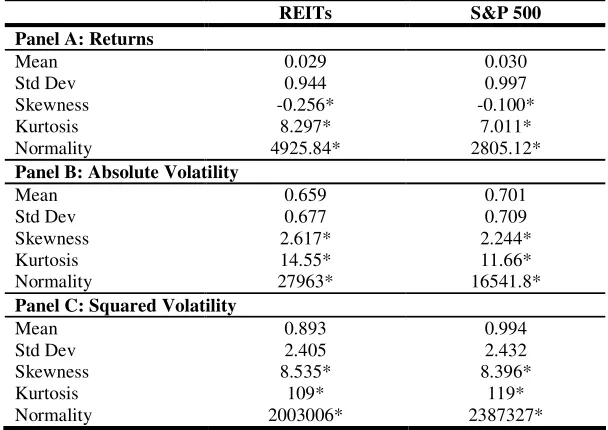
Some descriptive statistics of the respective series are outlined in Table 1 detailing the

first four moments of each series and a test for normality. Separate analysis is

completed for the returns series and the two proxies of volatility, absolute and squared

volatility. Starting with returns we find that the average daily returns of both series are

near zero but positive for the time frame analyzed suggesting that for the mainstream

equity market the 1990s boom has slightly outweighed the downturn at the start of

this decade. Accordingly, the reverse is true for the REIT sector, with their strong

recent performance outweighing the underperformance of the sector observed during

the late nineties. Overall however, the average risk of REITs approaches 1% and is

almost identical to the S&P. The time series behaviour of both series is given in

Figure 1. Here we can see the increase in volatility at the turn of the decade associated

with amongst other events, the fall out of the Asian crises and September 11, and the

technology bubble where equity markets in general exhibited greater turbulence and

very poor return performance. In the last couple of years the markets have settled

down to some degree.

In Table 1 evidence on higher moments of returns suggests negative skewness

recorded by both series suggesting that the weights of the large negative returns are

dominating their positive counterparts. Consistent with the literature, we also find

excess kurtosis suggesting that the series exhibit a fat-tailed property. Combining

these findings for skewness and kurtosis, we find that all series are non-normal using

the Jarque-Bera test statistic and therefore need to incorporate this property later in

Turning to the proxies of the volatility series, we first reiterate the findings for the

returns series, namely, that the REIT index exhibit similar volatility to the S&P and

behaviour over the sample period. Average volatility (regardless of proxy) in Table 1

are similar for both indexes. Looking at the plots in Figure 1 we see the behaviour of

the volatility associated with the series’ since 1990. We clearly see the volatility

clustering property where periods of high volatility or low volatility can remain

persistent for some time before switching. This property suggests that volatility on

any day is dependent on the previous day’s values and we will model this

phenomenon using a GARCH process that specifically incorporates long memory.

The lack of independence of either absolute or squared volatility is clearly seen by the

lack of normality and excess kurtosis reported in Table 1 for both series. We also get

strong positive skewness for all series that is reasonably similar across the series.

Comparing the two measures of volatility, we see that the magnitude of the squared

realizations dominate their absolute counterparts but that the squared values are more

prone to extreme outliers regardless of which series you examine.

4. Empirical Analysis

Our main focus in this paper is to examine the long memory properties of REITs and

it is to this issue that we now turn. We begin by discussing the autocorrelation plots;

followed by formal testing for long memory and determining the magnitude of the

long memory parameter, and finally we outline our findings from applying two

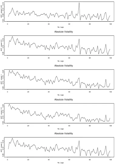
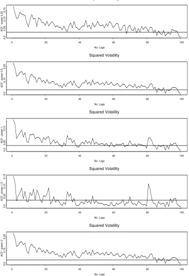
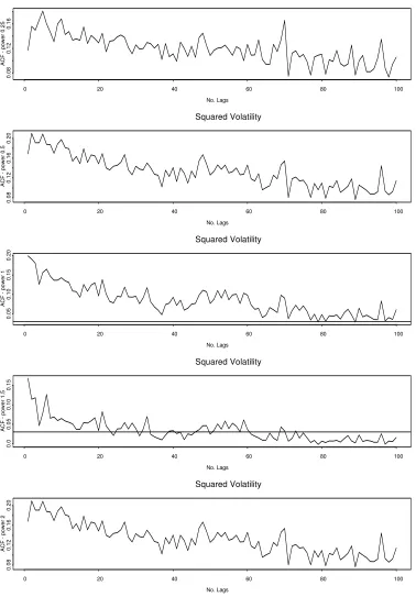
time-varying long memory volatility models. First, looking at dependence using the

autocorrelation function (ACF), we provide plots over 100 lags for the volatility series

and these are given in Figure 2 for absolute volatility and Figure 3 for squared

volatility.6 Ding et al. (1993) suggest that, as volatility is unobservable, the long

memory in equity data should be examined for different power transformations of the

volatility proxy series. We follow this suggestion by examining the volatility series

for 5 different power transformations [k=0.25, 0.5, 1, 1.5, 2]. This supports the

analysis of Beran (1994) in his seminal work in the area. In its strictest sense, the ACF

plots in Figures 2 and 3 do not offer conclusive evidence that REITs exhibit long

memory in volatility but are much more striking in their support for the property in

the broad market index. Moreover there is strong variation in the strength of the long

lower k. These findings are consistent for squared and absolute volatility. It is

noticeable that REITs appear to display less persistence in volatility than the general

market. The ACF plots for the S&P indexes report enhanced long memory. It can be

seen that in general the first lag for the REIT volatility ACF’s tends to be of a greater

magnitude but that the persistence reduces at a faster rate than for mainstream

equities.

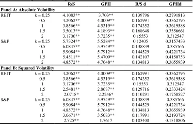
Table 2 reports details of the initial tests for long memory using the approaches

described in Section 2. There is extensive evidence of long memory in both the

absolute and squared volatility series’. This is consistent across all of the different

power transformations, although the effect is generally enhanced as k reduces,

particularly in the case of REITs. Furthermore, the magnitude of the test statistics is

generally lower for the REIT sector than for the S&P. The findings from fitting the

long memory volatility models are given in Table 3. The results generally show that

both the FIGARCH and FIEGARCH models provide good fits for the data, and are

broadly in line with expectations and the previously reported findings. The degree of

fractional integration, as measured by the d-values, is in the range of 0.3-0.4 for the

FIGARCH model for both series and is consistent with the previous empirical

evidence. In relation to the FIEGARCH model the significant negative leverage

coefficients also implies asymmetry in the long memory process with the greater

impact of negative shocks over positive shocks affecting not only immediate

volatility, but also on a persistent basis.

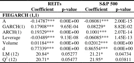
In the literature volume is seen as an important explanatory variable for time varying

volatility7. To investigate whether trading volume is important for the long memory

inherent in the volatility series we analyse the role of trading volume. In Figure 4 we

see the large increase in trading activity in equities and this is particularly pronounced

for REITs that had very low volume at the start of the sample. In Figure 5 we see that

the change in trading volume shows similar patterns to that of the price series,

namely, there is clustering of inactive (active) trading periods followed by active

(inactive) trading periods.

Taking the volume data we fit a FIEGARCH model and results are reported in Table 4

whether volume is an important mixing variable for long memory in volatility.

Trading volume is clearly an important explanatory variable for our conditional

volatility with a strong statistical significance. Also, economically a 1% change in

REIT volume is associated with a 0.01% change in its volatility and this effect is

approximately doubled for the S&P series. Interestingly, by including the change in

volume variable we see a major revision in the volatility specification with GARCH

and ARCH coefficients being considerably amended in comparison to the

FIEGARCH model results excluding volume. The main coefficients of the GARCH

process, whilst remaining significant, reduce in magnitude considerably, and provide

support for the hypothesis that volume and volatility are strongly related. The impact

of volume, however, is even more pronounced on long memory with the long memory

parameter, d, increasing to approximately 0.8 for both REITs and S&P series. Thus

the long memory characteristic is no longer present in the volatility series if we

include trading volume as an explanatory variable. Overall, changes (increases) in

volume are strongly associated with the long memory in property found in REIT (and

market) data.

5. Conclusion

This paper has examined the long memory properties in the volatility of the REIT

sector at daily frequencies. As the sector develops and daily trading volume increases

not only will interest in the daily dynamics in REITs increase but it will also in all

likelihood increase interest in derivative instruments based on the sector. The paper

illustrates that as with the general equity market volatility persistence occurs.

However, there is evidence that long memory in REIT volatility is not of the same

magnitude as that observed in the S&P 500 index. Moreover, changes in volume is an

References

Andersen, T.G. & Bollerslev, T. (1997a). Heterogeneous Information Arrivals and Return Volatility Dynamics: Uncovering the Long-Run in High Frequency Returns, Journal of Finance, 52, 975-1005.

Andersen, T.G. & Bollerslev, T. (1997b). Intraday Periodicity and Volatility Persistence in Financial Markets, Journal of Empirical Finance, 4, 115-158.

Andersen, T.G., Bollerslev, T., Diebold, F.X. & Labys, P. (2001). The Distribution of Realized Stock Return Volatility, Journal of Financial Economics, 61, 43-76.

Baillie, R.T. & DeGennaro, R.P. (1990). Stock Returns and Volatility, Journal of Financial and Quantitative Analysis, 25, 203-214.

Baillie, R.T. (1996). Long Memory Processes and Fractional Integration in Econometrics,

Journal of Econometrics, 73, 5-59.

Baillie, R.T., Bollerslev, T. & Mikkelsen, H.O. (1996). Fractionally Integrated Generalized Conditional Heteroskedasticity, Journal of Econometrics, 74, 3-30.

Beran, J. (1994). Statistics for Long-Memory Processes, Chapman & Hall: New York.

Black, F. (1976). Studies in Stock Price Volatility Changes, Proceedings of the 1976 Business Meeting of the Business and Economics Statistics Section, American Statistical Association, 177-181.

Bollerslev, T., & Mikkelsen, H.O. (1996). Modeling and Pricing Long Memory in Stock Market Volatility. Journal of Econometrics, 73, 151-184.

Bredin, D., O’Reilly, G. & Stevenson, S. (2008). Monetary Shocks and REIT Returns,

Journal of Real Estate Finance & Economics, forthcoming.

Breidt, F.J., Crato, N. & deLima, P. (1998). On the Detection and Estimation of Long-Memory in Stochastic Volatility, Journal of Econometrics, 83, 325-348.

Cotter, J. (2005). Uncovering Long Memory in High Frequency UK Futures. European Journal of Finance, 11, 325-337.

Cotter, J. & Stevenson, S. (2006). Multivariate Modeling of Daily REIT Volatility. Journal of Real Estate Finance and Economics.32, 305-325.

Davidian, M., & Carroll, R. J. (1987). Variance Function Estimation, Journal of the American Statistical Association, 82, 1079-1091.

Deo, R. S. & Hurvich, C. M. (2000). On the Periodogram Regression Estimator of the Memory Parameter in Long Memory Stochastic Volatility Models, New York University, Mimeo.

Devaney, M. (2001). Time-Varying Risk Premia for Real Estate Investment Trusts: A GARCH-M Model, Quarterly Review of Economics & Finance, 41, 335-346.

Ding, Z., Granger, C.W.J., & Engle, R.F. (1993). A Long Memory Property of Stock Returns,

Journal of Empirical Finance, 1, 83-106.

Ding, Z. & Granger, C.W.J. (1996). Modeling Volatility Persistence of Speculative Returns,

Journal of Econometrics, 73, 185-215.

Engle, R.F. (1982). Autoregressive Conditional Heteroskedasticity with Estimates of the Variance of UK Inflation, Econometrica, 50, 987-1008.

Engle, R. F. and Ng, V. (1993). Measuring and testing the impact of news on volatility,

Journal of Finance, 48, 1749-1778.

Geweke, J. & Porter-Hudak, S. (1983). The Estimation and Application of Long Memory Time Series Models, Journal of Time Series Analysis,4, 221-238.

Hurst, H. E. (1951). Long Term Storage Capacity of Reservoirs, Transactions of the American Society of Civil Engineers, 116, 770-799.

Kleiman, R.T., Payne, J.E. & Sahu, A.P. (2002). Random Walks and Market Efficiency: Evidence from International Real Estate Markets, Journal of Real Estate Research, 24, 279-297.

Lamoureux, C. G. & Lastrapes, W. D. (1990). Heteroskedasticity in stock return data: volume versus GARCH effects, Journal of Finance, 45, 221-229.

Lo, A. (1991). Long Memory in Stock Market Prices, Econometrica, 59, 1279-1313.

Lobato, I. N. & Savin, N.E. (1998). Real and Spurious Long-Memory Properties of Stock-Market Data, Journal of Business and Economic Statistics, 16, 261-268.

Najand, M. & Lin, C. (2004). Time Varying Risk Premium for Equity REITs: Evidence from Daily Data, Working Paper, Old Dominion University.

Nelson, D. B. (1991). Conditional Heteroskedasticity in Asset Returns: A New Approach.

Econometrica, 59, 347-370.

Scholes, M. and Williams, J. (1977). Estimating Beta From Non-Synchronous Data, Journal of Financial Economics,5, 309-327.

Stevenson, S. (2002a). An Examination of Volatility Spillovers in REIT Returns, Journal of Real Estate Portfolio Management, 8, 229-238.

Stevenson, S. (2002b). Momentum Effects and Mean Reversion in Real Estate Securities,

Journal of Real Estate Research, 23, 48-65.

Taylor, S.J. (1986). Modeling Financial Time Series, Wiley: London.

Taylor, S.J. (2000) Consequences for Option Pricing of a Long Memory in Volatility, Working Paper, University of Lancaster.

Tables & Figures

Figure 1: Time Series Plots of Daily Series

REITS R e tu rn s

1990 1994 1998 2002 2006

-8

0

6

1990 1994 1998 2002 2006

-8

0

6

1990 1994 1998 2002 2006

0

2

4

6

8

1990 1994 1998 2002 2006

0

2

4

6

8

1990 1994 1998 2002 2006

0

2

0

4

0

1990 1994 1998 2002 2006

0

2

0

4

0

Table 1: Summary Statistics for Daily Series

REITs S&P 500

Panel A: Returns

Mean 0.029 0.030

Std Dev 0.944 0.997

Skewness -0.256* -0.100*

Kurtosis 8.297* 7.011*

Normality 4925.84* 2805.12*

Panel B: Absolute Volatility

Mean 0.659 0.701

Std Dev 0.677 0.709

Skewness 2.617* 2.244*

Kurtosis 14.55* 11.66*

Normality 27963* 16541.8*

Panel C: Squared Volatility

Mean 0.893 0.994

Std Dev 2.405 2.432

Skewness 8.535* 8.396*

Kurtosis 109* 119*

Normality 2003006* 2387327*

Figure 2a: Plots of Autocorrelation Values for REIT Daily Absolute Volatility Absolute volatility No. Lags A C F p o w e r 0 .2 5

0 20 40 60 80 100

0 .0 0 .0 4 0 .0 8 Absolute Volatility No. Lags A C F p o w e r 0 .5

0 20 40 60 80 100

0 .0 0 .0 5 0 .1 0 0 .1 5 Absolute Volatility No. Lags A C F p o w e r 1

0 20 40 60 80 100

0 .0 0 .1 0 0 .2 0 Absolute Volatility No. Lags A C F p o w e r 1 .5

0 20 40 60 80 100

0 .0 0 .1 0 0 .2 0 Absolute Volatility No. Lags A C F p o w e r 2

0 20 40 60 80 100

0 .0 0 .0 5 0 .1 0 0 .1 5

Figure 2b: Plots of Autocorrelation Values for S&P Daily Absolute Volatility Absolute volatility No. Lags A C F p o w e r 0 .2 5

0 20 40 60 80 100

0 .0 4 0 .0 8 0 .1 2 0 .1 6 Absolute Volatility No. Lags A C F p o w e r 0 .5

0 20 40 60 80 100

0 .0 8 0 .1 2 0 .1 6 Absolute Volatility No. Lags A C F p o w e r 1

0 20 40 60 80 100

0 .0 8 0 .1 2 0 .1 6 0 .2 0 Absolute Volatility No. Lags A C F p o w e r 1 .5

0 20 40 60 80 100

0 .0 5 0 .1 0 0 .1 5 0 .2 0 Absolute Volatility No. Lags A C F p o w e r 2

0 20 40 60 80 100

0 .0 8 0 .1 2 0 .1 6

Figure 3a: Plots of Autocorrelation Values for REIT Daily Squared Volatility Squared volatility No. Lags A C F p o w e r 0 .2 5

0 20 40 60 80 100

0 .0 0 .0 5 0 .1 0 0 .1 5 Squared Volatility No. Lags A C F p o w e r 0 .5

0 20 40 60 80 100

0 .0 0 .1 0 0 .2 0 Squared Volatility No. Lags A C F p o w e r 1

0 20 40 60 80 100

0 .0 0 .0 5 0 .1 5 Squared Volatility No. Lags A C F p o w e r 1 .5

0 20 40 60 80 100

0 .0 0 .0 5 0 .1 0 0 .1 5 Squared Volatility No. Lags A C F p o w e r 2

0 20 40 60 80 100

0 .0 0 .1 0 0 .2 0

Figure 3b: Plots of Autocorrelation Values for S&P Daily Squared Volatility Squared volatility No. Lags A C F p o w e r 0 .2 5

0 20 40 60 80 100

0 .0 8 0 .1 2 0 .1 6 Squared Volatility No. Lags A C F p o w e r 0 .5

0 20 40 60 80 100

0 .0 8 0 .1 2 0 .1 6 0 .2 0 Squared Volatility No. Lags A C F p o w e r 1

0 20 40 60 80 100

0 .0 5 0 .1 0 0 .1 5 0 .2 0 Squared Volatility No. Lags A C F p o w e r 1 .5

0 20 40 60 80 100

0 .0 0 .0 5 0 .1 0 0 .1 5 Squared Volatility No. Lags A C F p o w e r 2

0 20 40 60 80 100

0 .0 8 0 .1 2 0 .1 6 0 .2 0

Table 2: Long Memory Diagnostics for Daily Series

R/S GPH R/S d GPHd

Panel A: Absolute Volatility

REIT k = 0.25 4.1083** 3.703** 0.139796 0.2791813

0.5 4.2062** 4.0009** 0.162991 0.3362795

1 3.8566** 4.5319** 0.174352 0.3619588

1.5 3.5013** 4.1893** 0.168648 0.3556661

2 3.1706** 3.7235** 0.15553 0.312547

S&P k = 0.25 5.7324** 5.5284** 0.12405 0.3157433

0.5 6.0847** 5.9749** 0.138839 0.385766

1 5.9084** 5.7912** 0.144529 0.4221734

1.5 5.4511** 5.4709** 0.142107 0.4150753

2 4.8572** 4.7648** 0.134813 0.3655939

Panel B: Squared Volatility

REIT k = 0.25 4.2062** 4.0009** 0.162991 0.3362795

0.5 3.8566** 4.5319** 0.174352 0.3619588

1 3.1706** 3.7235** 0.15553 0.312547

1.5 2.5481** 2.8687** 0.129716 0.2333424

2 2.0718* 2.2246* 0.110291 0.1758527

S&P k = 0.25 6.0847** 5.9749** 0.138839 0.385766

0.5 5.9084** 5.7912** 0.144529 0.4221734

1 4.8572** 4.7648** 0.134813 0.3655939

1.5 3.6671** 3.5083** 0.117991 0.2193724

2 2.725** 1.7617 0.103408 0.1310806

Table 3: Fractionally Integrated GARCH Models for Daily Return Series

REITs S&P 500

Coefficient p-value Coefficient p-value Panel A: FIGARCH (1,1)

A 0.04641*** 3.66E-06 0.02803*** 2.10E-07

GARCH(1) 0.50543*** 1.01E-11 0.54397*** 0.00E+00

ARCH(1) 0.37822*** 1.69E-08 0.18921*** 8.22E-15

d 0.3175*** 0.00E+00 0.39632*** 0.00E+00

LM (12) 20.9* 0.05189 7.942 0.7896

Q2 (12) 20.29* 0.06178 20.32* 0.06127

Panel B: FIEGARCH (1,1)

A -0.24867*** 0.00E+00 -0.10651*** 0.00E+00

GARCH(1) 0.13449** 2.72E-02 0.452*** 7.38E-08

ARCH(1) 0.33099*** 0.00E+00 0.13623*** 0.00E+00

Leverage -0.05662*** 1.41E-08 -0.0983*** 0.00E+00

d 0.59397*** 0.00E+00 0.63067*** 0.00E+00

LM (12) 17.94 0.1176 9.205 0.6853

Q2 (12) 17.61 0.1279 9.118 0.6928

Figure 4: Time Series Plots of Daily Volume Series

REITS

V

o

lu

me

Time

1990 1991 1992 1993 1994 1995 1996 1997 1998 1999 2000 2001 2002 2003 2004 2005 2006

1

0

0

0

0

5

0

0

0

0

S&P

V

o

lu

me

Time

1990 1991 1992 1993 1994 1995 1996 1997 1998 1999 2000 2001 2002 2003 2004 2005 2006

5

0

0

0

0

0

2

5

0

0

0

0

0

Figure 5: Time Series Plots of Daily Change in Volume Series

REITS

%

V

o

lu

m

e

Time

1990 1991 1992 1993 1994 1995 1996 1997 1998 1999 2000 2001 2002 2003 2004 2005 2006

-1

5

0

-5

0

5

0

1

5

0

S&P

%

V

o

lu

m

e

Time

1990 1991 1992 1993 1994 1995 1996 1997 1998 1999 2000 2001 2002 2003 2004 2005 2006

-1

5

0

-5

0

0

5

0

1

0

0

Table 4: Fractionally Integrated EGARCH Model with Volume

REITs S&P 500

Coefficient p-value Coefficient p-value FIEGARCH (1,1)

A -0.14787*** 0.00E+00 -0.08081*** 2.00E-15

GARCH(1) 0.17908*** 9.65E-04 0.08229* 8.82E-02

ARCH(1) 0.19329*** 0.00E+00 0.1001*** 2.07E-14

Leverage -0.03489*** 9.13E-08 -0.06085*** 1.45E-13

Volume 0.01184*** 0.00E+00 0.02012*** 0.00E+00

d 0.77339*** 0.00E+00 0.86554*** 0.00E+00

LM (12) 20.84* 0.05277 21.21* 0.04734

Q2 (12) 20.71* 0.05477 21.95* 0.03811

Figure 6: Time Series Plots of FIEGARCH Daily Conditional Volatility Series REITS F IE G A R C H C o n d it io n a l V o la ti lit y Time 19901991199219931994199519961997199819992000200120022003200420052006 0 .5 1 .5 2 .5 3 .5 S&P F IE G A R C H C o n d it io n a l V o la ti lit y Time 19901991199219931994199519961997199819992000200120022003200420052006 0 .5 1 .0 1 .5 2 .0 2 .5 3 .0 3 .5

Endnotes:

1

Two recent papers to have examined persistence and mean reversion in REIT and international real estate security returns are Kleiman et al. (2002) and Stevenson (2002b).

2

As volatility is a latent unobservable variable proxies of volatility such as absolute and squared returns are examined in the literature.

3

For an excellent treatment of long memory processes see Beran (1994).

4

Extensions of the Hurst (1951) R/S statistic involve replacing the sample standard deviation of the series, Z, with the square root of the Newey-West estimate of the long run variance.

5

One such example of a relatively successful application of standard GARCH models is the application of the APARCH model (see Cotter, 2005; for an example). The APARCH specification, developed by Ding et al. (1993) nests seven commonly applied GARCH models. However, the specification has an exponential decline structure that shows strong dependence but is not fully consistent with the long memory decline structure.

6

We also examine dependence of returns formally through long memory tests and informally through ACF plots. In line with previous studies we find negligible evidence to support the presence of long memory of returns. Results are available on request.

7

See Lamoureux & Lastrapes (1990). They find that trading volume reflects the dependence in information flows to the market that feeds directly into price volatility.

8