Social Network Capital, Economic Mobility and Poverty Traps

(1)

Munich Personal RePEc Archive

Social Network Capital, Economic

Mobility and Poverty Traps

Chantarat, Sommarat and Barrett, Christopher B.

January 2008

Online at

https://mpra.ub.uni-muenchen.de/6841/

(2)

Social Network Capital, Economic Mobility and Poverty Traps

†

Sommarat Chantarat and Christopher B. Barrett

§

January 2008 revision

Abstract

The paper explores the role social network capital might play in facilitating poor agents’ escape from poverty traps. We model and simulate endogenous network formation among households heterogeneously endowed with both traditional and social network capital who make investment and technology choices over time in the absence of financial markets and faced with multiple production technologies featuring different fixed costs and returns. We show that social network capital can serve as either a complement to or a substitute for productive assets in facilitating some poor households’ escape from poverty. However, the voluntary nature of costly social network formation also creates both involuntary and voluntary exclusionary mechanisms that impede some poor households’ exit from poverty. Through numerical simulation, we show that the ameliorative potential of social networks therefore depends fundamentally on broader socioeconomic conditions, including the underlying wealth distribution in the economy, that determine the feasibility of social interactions and the net intertemporal benefits of social network formation. In some settings, targeted public transfers to the poor can crowd-in private resources by inducing new social links that the poor can exploit to escape from poverty.

JEL Classification Codes: D85, I32, O12, Z13

Keywords: social network capital, endogenous network formation, poverty traps, multiple equilibria, social isolation, social exclusion, crowding-in transfer

© Copyright 2007 by Sommarat Chantarat and Christopher B. Barrett. All rights reserved. Readers may make verbatim copies of this document for non-commercial purposes by any means, provided that this copyright notice appears on all such copies.

†

We thank Gary Fields, Matt Jackson, Annemie Maertens, Flaubert Mbiekop, Tewodaj Mogues, Ian Schmutte, Fernando Vega-Redondo and seminar participants at Cornell University, Ohio State University, NEUDC 2006 and the Royal Economic Society Annual Conference 2007 for helpful comments on earlier versions. Any remaining errors are ours alone.

§

(3)

1

Social Network Capital, Economic Mobility and Poverty Traps

1. Introduction

The persistent poverty widely observed in developing countries has motivated much

research on poverty traps into which households may fall and from which they have

difficulty escaping. The fundamental feature of most poverty trap models centers on the

existence of financial market imperfections that impede investment in productive assets or

technology, and thus prevent households with poor initial endowments from reaching

higher-level equilibria in systems characterized by multiple equilibria.1 Meanwhile, a parallel literature emphasizes multiple pathways through which social network capital

might facilitate productivity growth, technology adoption and access to (informal)

finance.2 However, various studies also document the existence of exclusionary mechanism that can effectively prevent some poor from utilizing social networks to

promote growth.3 Advances in understanding the nature and limits of social network capital formation could offer insights into whether and how poor households might avoid

or escape poverty traps. There have been some notable recent efforts to make these links

explicit.4

This paper further explores the intersection between poverty traps and social

networks by studying the mechanisms by which endogenous social network capital can

facilitate or impede poor households’ escape from persistent poverty and the conditions

that may affect such mechanisms. While some empirical studies – e.g., Narayan and

Pritchett (1999) – find that social network capital effectively serves as a substitute for real

capital in mediating economic mobility, others, such as Adato et al. (2006), suggest that

accumulation of social network capital proves ineffective for households at the bottom of

the economic pyramid in highly polarized economies. What roles might social network

capital play in fostering or impeding the poor’s economic mobility? Why might

1

Examples include Loury (1981), Banerjee and Newman (1993), Galor and Zeira (1993), Dercon (1998), and Mookherjee and Ray (2002, 2003). See Azariadis and Stachurski (2005) or Carter and Barrett (2006) for helpful reviews of key threads in the poverty traps literature.

2

Dasgupta and Serageldin (2000) and Durlauf and Fafchamps (2004) offer excellent reviews.

3

For example, Adato et al. (2006), Mogues and Carter (2005) and Santos and Barrett (2006), among others.

4

(4)

2

endogenous social network formation help some poor households but not others? What

determines the poverty reduction potential of social networks? In this paper we develop a

simple, stylized optimization model and use simulations to elicit the quite mixed effects of

social network capital on poor households’ well-being dynamics in order to answer these

questions.

The basic structure and intuition of our model runs as follows. Households

heterogeneously endowed with privately owned capital assets and social network capital –

from endowed (e.g., parents’) social networks – choose production technologies,

consumption, and investment in assets and in social relationships with others in the

economy (that confer future social network capital) so as to maximize their lifetime

utility. We assume that social networks are costly to establish and maintain, have no

intrinsic value and only function to provide access to partners’ (at least partially

nonrivalrous) capital that can be used as productive input in the high-return technology.

Social networks form endogenously based on mutual consent and result from optimal

strategic interaction among all households in an economy. We simplify the setting by

assuming perfect information and no financial markets.

In this setting, analogous to other poverty traps models, some initially poor

households will be caught in a low-level equilibrium because they lack access, through

either endowments, markets or social mechanisms, to the productive assets needed in

order for the most productive technology available to be the households’ optimal choice,

albeit perhaps after a period of initial investment. Initially poor households without such

access must resort to autarkic savings if they are to finance later adoption of the improved

technology. Some find such investment attractive and thereby climb out of poverty of

their own accord. Others find the necessary sacrifice excessive and optimally choose to

remain relatively unproductive and thus poor. A third subpopulation might find

bootstrapping themselves out of poverty unattractive, but will make the necessary

investment if they receive some help from others, i.e., social network capital becomes

necessary for an escape from persistent poverty. A fourth subpopulation is able and

willing to make the necessary investment autarkically, but will find it more attractive to

invest in social relations that offer a lower cost pathway to higher productivity. The

(5)

3

prospects, others with socially-mediated growth prospects, with social relations either

complementing or substituting for own capital in economic mobility, while still others

have no real growth prospects at all.

The tricky part of the analysis stems from the fact that (i) social networks represent

complex sets of dynamic relationships established non-cooperatively between mutually

consenting agents, and (ii) a given relationship or link’s net value to any agent depends on

the set of other links operational at the same time. Because the social network structure

thus evolves endogenously and depends fundamentally on the wealth distribution of the

underlying economy, the partitioning of the initially poor among the four subpopulations

just identified will vary in both cross-section and time series. This complex

interdependency in a setting with multiple and heterogeneous households poses an

analytical challenge, which we address using numerical simulations.

The remainder of the paper is structured as follows. Section 2 briefly summarizes

the empirical evidence on social network capital and key implications for endogenous

network formation in low-income economies relevant to this paper. Section 3 develops a

dynamic optimization model with endogenous network formation among heterogeneous

households, describes the simple non-convex production technology set and households’

unilateral decisions, and explains the game theoretic approach we use to characterize

endogenous network formation in this model. Section 4 then describes households’

equilibria for any equilibrium network that may arise in this stylized economy. We then

discuss the roles social networks play and the resulting patterns of economic mobility and

immobility using the distinguishable concepts of static and dynamic asset poverty

thresholds as a function of asset and social network capital. We also review the model’s

comparative statics. Section 5 illustrates these results and their implications by simulating

randomly generated economies to demonstrate different mobility patterns of households

in any economy and of households with identical initial endowments in different

economies. The simulations also allow us to show, in section 6, how endogenous social

network formation can overturn familiar policy implications generated by models without

endogenous social interactions, as when public transfers to the poor no longer crowd-out

private transfers but can, instead, crowd them in by inducing the creation of new social

(6)

4

2. Social network capital

Despite its elusive definitions and applications, a rapidly growing literature on

“social capital” emphasizes its potential to obviate market failures in low-income

communities. Durlauf and Fafchamps (2004) distinguish between two broad concepts of

social capital identifiable in the literature. First, social capital is sometimes referred to as a

stock of trust and associated attachment(s) to a group or to society at large that facilitate

coordinated action and the provision of public goods (Coleman 1988, Putnam et al.1993).

A second conceptualization treats social capital as an individual asset conferring private

benefits (Onchan 1992, Berry 1993, Townsend 1994, Foster and Rosenzweig 1995,

Fafchamps 1996, Ghosh and Ray 1996, Kranton 1996, Barr 2000, Bastelaer 2000, Carter

and Maluccio 2002, Conley and Udry 2002, Fafchamps and Minten 2002, Isham 2002,

Fafchamps 2004, Bandiera and Rasul 2006, Moser and Barrett 2006). We employ the

second conceptualization, which is sometimes referred to as “social network capital” so as

to emphasize that households gain from linking with others to form social networks for

mutual benefit (Granovetter 1995a, Fafchamps and Minten 2002).

The literature identifies various pathways through which social networks might

mediate economic growth: improved information flow and informal access to finance for

technology adoption, market intelligence or contract monitoring and enforcement, access

to loans or insurance, or provision of friendship or other intrinsically valued services. For

simplicity, this paper considers the setting where the sole function of a social network is

to provide access to link partners’ (at least partially nonrivalrous) productive assets, which

are essential for adoption of the high-return technology. Intuitively, this can be understood

as sharing or borrowing tools, equipment or even animal or human labor, obtaining

nonrivalrous capital-specific information, etc., which are costly, productive inputs in

high-return production.5 For example, a farmer’s social link to another farmer might afford free access to the latter’s tractor or at least to information that reduces tractor acquisition or

operating costs if the farmer opts to buy a tractor himself. The social network in our

5

(7)

5

setting thus has purely instrumental value in allowing one to accumulate social network

capital, naturally defined as socially-mediated access to others’ productive assets.

Social network capital is assumed to be productive only in the high-return

production, but incompatible with the low-return, subsistent level of production. It is thus

(imperfectly) substitutable for traditional, privately possessed capital.

The prospective benefits of social network capital create material incentives to

establish social relations with others, even when it is costly to establish and maintain such

relationships. The formation of a social network of bilateral relationships is thus a form of

investment, akin to more conventional investment in traditional financial, natural or

physical capital.

Social networks necessarily evolve endogenously. A small but growing literature

demonstrates this empirically in the case of poor agrarian communities (Conley and Udry

2001, Fafchamps and Minten 2001, DeWeerdt 2004, Santos and Barrett 2005, Fafchamps

and Gubert 2007). Because social networks are (at least partly) the consequences of

individual’s cost-benefit calculus with respect to prospective links with others, and those

costs and benefits depend on social distance and the underlying structure of the economy,

network structure is highly variable.

Theorists have for some time offered insightful strategic models of endogenous

network formation, building on seminal works by Aumann and Myerson (1988), Myerson

(1991) and Jackson and Wolinsky (1996), among others. In recent years, formal

theoretical models of network formation have been increasingly applied in development

economics (Calvό-Armengol and Jackson 2004, Conley and Udry 2005, Genicot and Ray 2005, Mogues and Carter 2005, Bloch et al. 2006). Nonetheless, most of the social

networks studies related to economic development have been empirical, and in aggregate

strongly suggest that not everyone benefits from social networks and that there exist

patterns to failures to form network links (Durlauf and Fafchamps 2004). For example,

Figueroa et al. (1996) point out that social exclusion has become a very active subject of

debate concerning poverty in Europe. Carter and May (2001) and Adato et al. (2006)

show that the voluntary and involuntary exclusion of poorer black households from the

social networks of wealthier whites in South Africa has prolonged the legacy of apartheid

(8)

6

to entry into remunerative livelihoods. Santos and Barrett (2006) find that asset transfers

through social networks in southern Ethiopia systematically exclude poorer households,

corroborating insights from anthropologists and historians studying similar systems across

rural Africa.

Nonrandom patterns of unformed latent social links within a society reflect choices

made by individuals to forego prospective relationships. We refer to the situation where

an individual opts not to seek out partners as “social isolation”, reflecting voluntary

self-selection out of prospective networks.6 In other cases, individuals desire links with others but are rebuffed by prospective partners, resulting in involuntary “social exclusion”.7 We

demonstrate below how patterns of social exclusion and isolation may turn fundamentally

on the initial wealth distribution in an economy, with significant consequences for the

growth prospects for the poor.8 In this way, models of endogenous social network capital as an input into productivity growth provide a natural link between the social networks

literature and that relating income distribution to economic growth.9 Having situated this paper in the broader literature and laid out the core intuition and concepts, we now explain

our stylized model in detail.

3. A simple dynamic optimization model with endogenous network formation

Assume n households exist in an economy, N =

(

1,2,...,n

)

. Each lives for two periods,10 t=0,1. Each household i is initially endowed with two types of assets:

traditional productive capital, denoted A_i₀, representing a one-dimensional aggregate index measure of physical, natural, human and financial capital, and social network

6

Postlewaite and Silverman (2005), Kaztman (2001), Barry (1998), Wilson (1987), among others, similarly use the concept and term “social isolation” to reflect voluntary non-participation in a society’s institutions.

7

Note that we use the term “social exclusion” very precisely, especially as compared to the literature on social exclusion as, more generally, “inability of a person to participate in basic day-to-day economic and social activities of life” (Chakravarty and D’Ambrosio 2006, p.397), as the term is used by, among others, Room (1995), Atkinson (1998), Atkinson et al. (2002), and Bossert et al. (2007).

8

We only directly refer to social isolation and social exclusion with respect to those agents who remain poor over time and do not establish social networks. Extension to those non-poor who similarly do not link with others is straightforward, but omitted in the interest of focus on the paper’s core poverty traps theme.

9

See, for example, Galor and Zeira (1993) or Mookherjee and Ray (2000), as well as the excellent review by Aghion et al. (1999).

10

(9)

7

capital, denoted S_i₀, referring to the traditional capital that might be acquirable from others in the endowed (e.g., parents’) social network. There is thus just one type of

individually owned asset, but people can have access to it directly through private

ownership or indirectly through their social network. The economy’s initial endowment

distribution is denoted by

λ

(

A₀,S₀

)

. Households’ preferences are identical, with utility derived solely from consumption, as is the set of available production technologies to

generate income from one’s capital stock.

3.1 Production technology set

The available production technology set in this economy consists of two

technique-specific production functions that generate low and high income at any period t, Y_tL and

H t

Y , respectively, through

( )

t

L L

t f A

Y = (1)

(

t ( t)

)

H H

t f A F S

Y = − with F

( )

St ≥0, −1<F′

( )

St <0 and F

( )

∞ =0. (2)

Technology L is a low-cost, low-return technique that everyone can afford. Technology H

is a high-return technology with a fixed cost entry barrier, F

( )

S_t ≥0. Greater capital is thus required to make technology H attractive because one has to cover the fixed cost of operation (i.e., this is not a one-time sunk cost of adoption). Social network capital

reduces the fixed cost of using the high-return technology and is thus an imperfect

substitute for owned capital.

Each production technology fulfills standard curvature conditions. For net

productive assets, NA_tH ≡ A_t −F

( )

S_t ≥0 and NA_tL ≡ A_t ≥0, (almost everywhere)

twice-differentiable functions f_H

(

NA_tH

)

and f_L

( )

NA_tL follow

( )

0 = _L

( )

0 =0

H f

f (3)

( )

₌_∞

∂ ∂ = ∂

∂

L t L H t H

NA f NA

f 0 0

and

( )

=0

∂ ∞ ∂ = ∂

∞ ∂

L t L H t H

NA f NA

f

(10)

8

(

)

0 ) ( 2 2 ≤ ∂ ∂ H t H t H NA NA f

and

( )

0 ) ( 2 2 ≤ ∂ ∂ L t L t L NA NA f (5)

(

)

( )

0 | | ≥ ∂ ∂ ≥ ∂ ∂ = = L NA j

t L t L j NA H t H t H t t NA NA f NA NA f j

∀ . (6)

In each period t, therefore, a household i’s aggregate production function can be described as

Max

Y_it = [ Y_itH,Y_itL] = Max[ f_H

(

A_it −F(S_it)

)

, f_L

( )

A_it ] (7) which yields a non-convex production set, with locally increasing returns in the

neighborhood of A

( )

S_it , the asset threshold beyond which a household will optimally switch to the high-return production technology. A

( )

Sit thus satisfies

H

f [A

( )

S_it −F(S_it)] = f_L[A

( )

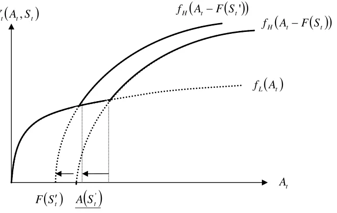
S_it ]. (8) Figure 1 presents this aggregate production function as an outer envelope of the two

specific production functions, with the threshold asset stock A

( )

S_it .11

Social network capital thereby reduces the private asset stock necessary to make

technology H optimal. As Sit increases, the high-return production function shifts in,

lowering the minimum asset threshold needed to make high-return production optimal,

i.e., A′

( )

S_it <0, which follows implicitly from (8) and the assumption that F(·) is decreasing in Sit. This effect is depicted in Figure 2.

An obvious implication is that the value of social network capital will vary across

households. For householdswith sufficient privately-held assets,A_kt ≥ A

( )

S_kt , adoption of

H is optimal regardless of their stock of social network capital, but Sit nonetheless reduces

the fixed costs they incur, thereby increasing the productivity of their asset stock. Their

investment incentives are thus driven by the relative costs of investment in social network

capital and traditional, privately held assets.

11

(11)

9

Social network capital is potentially most valuable for those households k who possess insufficient assets themselves to adopt H,Akt < A

( )

Skt , but who are “not too far”

in some sense from A

( )

S_kt so that investment in building social network capital can lower the critical threshold they face to the point that the high-return technology becomes

optimal in the future. Because social network capital has no value for those who do not

employ technology H, however, as one’s distance from A

( )

S_kt increases the prospective benefit from increased future social network capital eventually falls once it will not

suffice to bring the threshold down far enough, given the household’s current and

prospective asset stock. For such households, there is no incentive to invest in social

network capital, thus they will rationally self-select out of costly social relations, thereby

becoming socially isolated.

3.2 Household utility maximization

A household i derives utility solely from consumption each period, maximizing

( )

i0

( )

i1

i u C uC

U = +

ρ

(9)

where

ρ

is the discount factor. We further assume there are no financial markets, thus

autarkic saving is the only investment strategy. A subsistence consumption constraint

applies such that for any level of consumption necessary for survival C >0;

−∞ =

) (C_it

u for any C_ir <C and r≤t. (10) This puts a minimal limit on the intertemporal consumption tradeoff available to the

household by permanently penalizing extremely low consumption in any period.

In period 0, a household i with endowments

(

A_i₀,S_i₀

)

optimally chooses a production technology and allocates the resulting income from production among

(12)

10

and the column vector of costs the household has to incur to establish or maintain12 these relationships (Ki).13

Note that the household incurs costs in period 0 for establishing network Xi0, but it

derives no immediate benefits. The laws of motion mapping initial endowments into

stocks at the beginning of period 1 depreciate Ai₀ and Si0 at rates δA and

δ

S,

respectively, while period 0 investments add to the stock of both assets. The new stock of

social network capital is a function of the household’s social network at the end of period

0 and the benefit function (Bi) that maps proportion of assets held by members of its

established network into social network capital, as described in section 4. In period 1, the

household again chooses the optimal production technology and consumes all the

resulting income.14

A key distinction between A and S is that the household unilaterally decides the stock of traditional capital it will own, but it does not unilaterally decide on its social

network because each social link involves bilateral decisions by both prospective partners.

The household’s social network is therefore the product of optimal social interactions,

taking into consideration everyone in the economy’s network preferences. A household’s

utility maximizing network might therefore prove infeasible because its preferred link

partners do not have reciprocal desires for an active link. In modeling the household’s

decision, we thus defineX_iu₀ = X_i₀

(

X₋_i₀

)

as household i’s desired, unilateral network choice conditional on others’ choices, denoted by X₋_i₀.

12

Because, realistically, some agents begin with inherited social network capital – e.g., familial ties with biological relatives and parents’ close associates – we assume that household’s endowed social network capital exists independent of its de novo network link choices, subject only to a uniform rate of depreciation of the social network capital – think of this as mortality or out-migration of pre-existing ties.

13

Both Ki and Xi0 are described in more detail in the next section.

14

(13)

11

( ) ( ) ( )

{

Max

u

}

i i u i i u i

i X I X C X

C₀ ₀, ₀ ₀, ₁ ₀

( )

u i i X

V* ₀

Specifically, the indirect utility that household i with endowments

(

A_i₀,S_i₀

)

derives from a possible network choice u

i

X ₀ is simply

= u

( )

C_i₀ + ρu

( )

C_i₁ (11)

subject to:

(

)

i

u i i i i i

i Y A S I X K

C₀ ≤ ₀ ₀, ₀ − ₀ − ₀

(

)

0 0

1 1 A i i

i A I

A = −

δ

+

(

)

i

u i i S

i S X B

S₁ = 1−

δ

₀ + ₀

(

1 1

)

1 1 i i , i i Y A S

C ≤

0 , ₁

1 i ≥ i A

S

. , ₁

0 C C

C_i _i ≥

The production function follows (7) and the subsistence constraint is incorporated into the

final constraint on consumption. Each household can perform intertemporal cost-benefit

calculus for any of their network choices conditional on choices of others. We now detail

the specifications for the endogenous network formation and the suitable equilibrium

concept in order to resolve this intertemporal optimization problem.

3.3 Endogenous network formation

Because the formation of links is a strategic decision affecting households’ optimal

consumption and investment decisions, we model network formation as a non-cooperative

game in which link formation is based on a binary process of mutual consent between

individuals who costlessly observe the current wealth distribution. Due to the multiplicity

of equilibria, many of which make little sense from a social network perspective, we

reduce the range of feasible equilibria through imposing two restrictions. The first follows

from the fact, well-established in sociology, that active social networks are primarily

formed among individuals already acquainted with one another. This implies a central role

for social distance in determining the net benefits of active link formation. We let social

distance affect the individual-specific costs and benefits of link formation in a way that

helps limit the range of prospective links to a domain over which they are most likely.

(14)

12

with perfect information, which allows us to find a subgame perfect Nash equilibrium

(SPNE) social network in this economy.

Social distance, feasible interactions and link-specific cost-benefit analysis

A broad literature suggests there exist boundaries to prospective social interactions.

Santos and Barrett (2005, 2006), among others, find that not everyone knows everyone

else, even in small, ethnically homogeneous rural settings in which households pursue the

same livelihood, and that knowing someone is effectively a precondition to establishing

an active link. Consistent with this, many models of network formation emphasize local

interactions within prescribed neighborhoods (Ellison 1993, Ellison and Fudenberg 1993,

Fagiolo 2001).

In our setting, each household is characterized by its universally observable

(

A₀,S₀

)

endowment. Thus each household can identify its social distance from every other

household in

(

A,S

)

space. As in Akerlof (1997) or Mogues and Carter (2005), we use the geometric distance between households’ endowments to reflect social distance,

( )

(

)

(

)

2

0 0 2

0 0

, j A_i A_j S_i S_j i

d = − +

α

− ; α ≥0, (12)

for any pair of households, i and j, where α establishes the relative weight of pre-existing social network capital in determining social distance. Conceptually, social distance

measures relative proximity between two households, which reflects the degree of

discomfort in their social interaction. It can thus serve as a proxy for the cost of

establishing and maintaining a social relationship.

Formally, a household i incurs total costs of X_i′₀K_i to establish its network of links

0 i

X , where Ki is a column vector of costs they have to incur to establish each active link.

To keep the analysis as general as possible, the economic cost to household i to establish a link with household j can be written as

( )

(

( )

)

_⎟⎟

⎠ ⎞ ⎜⎜ ⎝ ⎛ ⋅ =

0 0

,

i j i

A A j i d k j

K with k′>0 for d(i,j)≤d, k′=∞ otherwise. (13)

The idea is that it is easier to establish a link with people who are socially proximate,

(15)

13

costs, here specified such that the poorer partner incurs more costs in link formation. We

assume no economies of scale or scope in building networks.

The constant d reflects a social distance threshold beyond which social interaction

is not feasible.15 In our context, d is economy-specific but universal to each household in

the economy.16 It implicitly reflects physical and social barriers on the probability that

individuals meet and interact. A low d can represent an economy in which households cluster into many small groups of shared characteristics with low inter-group connectivity

or an economy characterized by significant ethnic, racial or religious discrimination or

physical isolation. A high d, on the other hand, allows for greater social interactions. The benefits to household i from the active links in its social network are reflected in the column vector Bi, mapping some proportion of its partners’ asset endowments into

augmentation of its social network capital next period. Specifically, the gross benefit to

household i from a link with household j follows

( )

(

_j₀, _i₀ _j₀

)

i j b A A A

B = − where 0<b₁′ <1 , −1<b₂′ <0 (14)

Implicitly, 0<b₁′ <1 emphasizes the nature of access to link partners’ (at least partially nonrivalrous) capital.17 This generalization is highly stylized but very intuitive. Some components of the composite asset are nonrivalrous (e.g., equipment-specific

knowledge). Others, such as tools and equipment, can be shared and thus used at different

time without materially affecting the owner’s (or other borrowers’) use, but perhaps with

degraded performance for the borrower (e.g., due to imperfect timing). Whether one

considers this unfettered, occasional or probabilistic access, the key is that i’s access to socially-mediated capital is increasing in the stock of links’ privately-held assets.

As with the costs of links, we assume that social network capital benefits are

link-specific and independent of all other links the household establishes. The social network

capital gained from a link is not symmetric to both members of the dyad for the simple

15

In the language of the networks literature,ddistinguishes between local and global interactions.

16

This assumption is reasonable give households’ identical preferences. The sensible extension of this context is to allow d to vary with other socioeconomic characteristics (e.g., initial endowments, groups).

17

(16)

14

reason that a poorer household can call on more resources from their richer partner than

vice versa. Extreme differences in wealth, however, may hinder mutual benefits, as

reflected in the second argument in (14). Intuitively, the specific capital of one partner

might be inappropriate to a partner employing quite different practices due to stark wealth

differences. More generally, the asymmetric specification of (14) fits the empirical pattern

that wealthy households are more likely to opt out of links with much poorer partners than

vice versa (Santos and Barrett 2005). In similar spirit, very poor households might not

find it attractive to link with far richer ones with whom they share little (Mogues and

Carter 2005).

Two fundamental points distinguish our network formation model from others. First,

costs and benefits of links are realized intertemporally.18 A household’s preference over possible networks, therefore, relies on its realized net intertemporal utility gains. Second,

household i’s decision to link with household j is interdependent with its decision to link with others. A link with one household might complement or substitute for links with

others. The multiple equilibria in our setting accentuate this interdependency because only

those households that can accumulate enough resources to make the high-return

production technology optimal will benefit from social network capital. Therefore, many

households’ valuation of a given link is conditional on their success in establishing other

links as well. To take into account these spillover possibilities, households’ network

strategies involve choosing among possible networks of links, instead of just myopically

considering each link separately.

We use the notation ij to describe the binary link between households i and j. According to (13), social links can be established within the feasible interaction space

determined by d. The network of household i, reflecting the combination of its binary links, is represented by the vector:

X_i =

(

x

( )

ij j∈N, j≠i,d(i, j)≤d

)

where x(ij)∈

{ }

0,1 . (15)

18

(17)

15

The binary index x

( )

ij is defined by joint agreement to establish a link,x

( )

ij =1, otherwise x

( )

ij =0. Household i’s set of all feasible networks can then be represented by

{ }

{

/ ( )∈ 0,1

}

=

Ω_i X_i x ij .

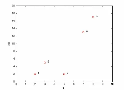
By way of illustration, consider an economy with N =

{

1,2,3,4,5

}

and the endowment distribution λ

(

A₀,S₀

)

illustrated in figure 3. For d =9, for example,

household 3’s network can be generally represented by

( )

⎟⎟ ⎟ ⎠ ⎞ ⎜ ⎜ ⎜ ⎝ ⎛ = 34 32 31 3 x x x

X with x

( ) { }

3k ∈ 0,1

for all k =1,2,4. Clearly interaction between 3 and 5 is not feasible because

) 5 , 3 (

d >d =9 . Hypothetically,

⎟ ⎟ ⎟ ⎠ ⎞ ⎜ ⎜ ⎜ ⎝ ⎛ = 0 0 1 3

X represents household 3’s network that consists

of only a link with household 1.

⎟ ⎟ ⎟ ⎠ ⎞ ⎜ ⎜ ⎜ ⎝ ⎛ = 1 1 1 3

X arises when 3 establishes links with everyone

with whom interaction is feasible, while

⎟ ⎟ ⎟ ⎠ ⎞ ⎜ ⎜ ⎜ ⎝ ⎛ = 0 0 0 3

X presents the case where household 3

has no links.

⎪ ⎭ ⎪ ⎬ ⎫ ⎪ ⎩ ⎪ ⎨ ⎧ ⎟ ⎟ ⎟ ⎠ ⎞ ⎜ ⎜ ⎜ ⎝ ⎛ ⎟ ⎟ ⎟ ⎠ ⎞ ⎜ ⎜ ⎜ ⎝ ⎛ ⎟ ⎟ ⎟ ⎠ ⎞ ⎜ ⎜ ⎜ ⎝ ⎛ ⎟ ⎟ ⎟ ⎠ ⎞ ⎜ ⎜ ⎜ ⎝ ⎛ ⎟ ⎟ ⎟ ⎠ ⎞ ⎜ ⎜ ⎜ ⎝ ⎛ ⎟ ⎟ ⎟ ⎠ ⎞ ⎜ ⎜ ⎜ ⎝ ⎛ ⎟ ⎟ ⎟ ⎠ ⎞ ⎜ ⎜ ⎜ ⎝ ⎛ ⎟ ⎟ ⎟ ⎠ ⎞ ⎜ ⎜ ⎜ ⎝ ⎛ = Ω 1 1 1 , 1 1 0 , 1 0 1 , 0 1 1 , 1 0 0 , 0 1 0 , 0 0 1 , 0 0 0

3 thus represents the set of all

feasible network.

The indirect utility Vi

( )

Xi *

associated with the network choice Xi

19

can naturally

be used to compare among household i’s feasible networks. And thus household’s preference over the feasible networks can be obtained by ranking their feasible networks

based on the correspondingVi

( )

Xi *

. Strategic interactions among all households in the

economy then involve households choosing their network of social links from the set of

19

The time index t=0is dropped here. In the next section, however, the optimal network is denoted as * 0 i

(18)

16

feasible ones using the resulting set of ranked networks, ΩRanked_i as their reaction function

in an extensive form game of link formation, which we now describe.

Linking game with perfect information

Because network link formation is a strategic decision affecting households’ optimal

consumption and investment decisions, it is natural to model network formation as a

non-cooperative game. The mutual consent requirement of link formation poses a hurdle,

however, to the use of any off-the-shelf solution technique, especially due to issues of

multiplicity and stability of equilibria (Jackson 2005). Reviewing seminal models of link

formation, Jackson (2005) concludes that the mutual consent requirement for link

formation implied either some sort of coalitional equilibrium concept or an extensive form

game with a protocol for proposing and accepting links in some sequence. As the purpose

of this paper is not to study the nature of network formation per se, but rather to use a

sensible equilibrium network concept to analyze the ways in which the resulting social

network capital mediates economic mobility, we opt for the latter approach and develop a

reasonable extensive form game of network formation with perfect information that yields

a SPNE network.

We model households attempting to establish their utility maximizing network as

players interacting over multiple rounds of link proposing, accepting and rejecting, using

Ranked i

Ω as their best response function. This extensive form game thus involves an

algorithm for proposing and accepting links that yields a sequential matching process.20 At the beginning of the game there are no pre-established links between any player

households.21 Initially, households consider their top-ranked network. They simultaneously propose to each of the other households with which they wish to link. The

link between two households is established if and only if (i) both agents propose to each

20

This specification is in the context of a matching game in the domain of a coalitional game, in which each household may be matched with many others. Our matching specification differs greatly, however, from Gale and Shapley’s (1962) original approach, which considers a two-sided one-to-one matching game in which members of two sides are referred to as Xs and Ys. It also differs from marriage models and the roommates problem in which individuals can match with only one partner.

21

Think of S0as reflecting one’s inherited links with an older generation and the network choice, Xi, as

(19)

17

other, and (ii) at least one of the two partners optimizes its network (i.e., has all of its

proposals accepted). Once a household optimizes its network, its game is concluded. For

any of its partners that do not likewise optimize their networks, these established links are

binding. Such partners continue to play the game, with their utility maximization now

constrained by the link commitment. All households that do not optimize their networks

in a proposal round move on to the next round, when they again simultaneously propose

to each of those households still active in the game with whom they wish to link in their

top-ranked still-feasible network (which must include any pre-existing link commitments

from prior rounds with households that have concluded play). The same link formation

rule is followed. The game then repeats itself if there remain households without

optimized networks. The entire history of offers, acceptances and rejections is known to

all households.

If no household can optimize its network in a specific stage, and thus no binding

link can be established, we assume that the poorest household (i.e., the one with lowest

A0) has to forego its top-ranked network and instead use its second-best network while the

rest still play their top-ranked networks. If still no one can optimize the network, the

second poorest household then sacrifices its first-best network and must make link

proposals to its second-best network while all richer households still play their first-best

strategy, and so on. The process of sequential matching continues until everyone

optimizes their networks following the protocol outlined above. For any preferences, the

process eventually stops because there exists a finite set of households in this economy.

This process results in a set of links. We will denote this set by g. Household i’s social network derived from this resulting set of link g can then be denotedXi

( )

g . The

payoff to each household i is then defined by the corresponding indirect utility

( )

(

X g

)

Vi i

*

. Given perfect information, this protocol generates a SNPE in pure strategies

(Selten 1975).

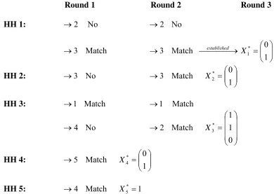
Figure 4 provides a numerical illustration of this algorithm and its SPNE for the five

player example economy from Figure 3. Note three interesting aspects of this proposed

game. First, even if proposals are matched, this does not guarantee the establishment of a

link. Binding links are established only if (at least) one partner optimizes its network. This

(20)

18

are governed by their preferences over their broader networks, as reflected in Ω_iRanked.

Second, households’ optimal networks in equilibrium are not necessarily their first-best

ones, due to the interactive nature of the link formation process and the spillovers inherent

to the process economywide. This creates a stark contrast vis-à-vis the optimality

conditions that would result from unilateral decisions regarding social network structure.

Third, the game’s SPNE network tends to favor those households able and/or preferring to

link with a small number of others.22

We then use 100 randomly generated economies to explore some simple properties

of this endogenous network formation. Appendix 2 reports the details of the baseline

parameterization of the model. Appendix 3 includes detailed results of sensitivity analysis

performed by varying some of the more important parameter values. Explicit examination

of other properties of this extensive game with large number of heterogeneous players is

very difficult23 and is not in the objective of this paper.

4. Households’ equilibria and patterns of economic mobility

Due to the mutual consent requirement for link formation, household i’s optimal network in the SPNE of the extensive form game just described constrains the optima for

each household in the economy, not just for i’s optimal technology choice, welfare, etc.

The equilibria of this model are, therefore, characterized by every household’s

accumulation decisions,

{

Xi Ii

}

_i 1,...,_n *

0 *

0, = , which determine current and future technology

choice, consumption levels, and thus each household’s level of well-being.

The preceding model specifications prepare us now to study how social network

capital influences households’ economic mobility through their optimal network

formation and capital accumulation decisions. We study a general case where each

22

This is illustrated in the simulation statistics in Appendix 1.Those for whom no links are feasible or who do not wish to establish any social links (i.e., socially isolated households) necessarily always get their first-best network. Thereafter, the proportion of households attaining their first-first-best network in equilibrium is declining monotonically in desired network size (Figure A2) and non-monotonically in feasible network size (Figure A1). This merely reflects that more complex networks are harder to establish.

23

(21)

19

household i, initially endowed with

(

A_i₀,S_i₀

)

, faces the unilateral intertemporal utility maximization problem (11) with the general instantaneous utility function:

( )

θ θ

−

= −

1

1 it it

C C

u ; 0≤θ <1, (16)

where θ determines the household’s willingness to shift consumption between periods.

The smaller is θ, the more slowly marginal utility falls as consumption rises, and so the

more willing the household is to allow its consumption to vary over time. We consider the

non-convex production technology set in each period t =0,1described in (7) in the general

Cobb-Douglas form

(

A S

)

Max

Y _it, _it = [

( )

1

(

( )

)

2

2 1 ,

α α

it it

it k A F S

A

k − ] , 0<α₁,α₂ <1,α₂ >α₁, 0k₁,k₂ > . (17) We specifically concentrate on the setting in which high-return production is always

preferable to the lower return technology. Without the borrowing constraint, every

household would gradually converge to this superior equilibrium, whether through

borrowing, autarkic savings, or both. The assumptions of constrained autarkic savings –

per (10) – and no borrowing thus lead to the existence of multiple equilibria, one of which

is the poverty trap associated with continued use of the low-return technology.

4.1 The benchmark case without a social network

We now analyze the benchmark case without social networks, in which the

household’s optimal welfare depends solely on its autarkic savings and accumulation

capacity. The next subsection then expands the analysis to consider the case in which

households can form social networks and explores how this affects economic mobility,

especially among those who might otherwise be trapped in poverty.

The case where Sit =0∀t, implying no functioning social network, replicates a traditional poverty traps model. The non-convex production set in (17) implies an asset

threshold A such that, at any period t, those with A_t ≥ A can optimally undertake high-return production.24 For simplicity’s sake, assume those who choose the low return technology (the first argument on the right-hand side of (17)) generate income that leaves

24

(22)

20

them poor while those who choose the high-return technology (the second argument on

the right-hand side of (17)) earn income that renders them non-poor. Thus threshold A

represents a static asset poverty line, which distinguishes current poor from non-poor. In any period t, the poor in our context are, therefore, those households with At < A, i.e.,

those currently undertaking low-return production.

Household i’s first-order conditions for an interior optimum thus potentially yield two equilibria: the low-level equilibrium (poverty trap) U_iL*

(

S_i₀ =0,X_i₀ =0

)

and the

high-level equilibrium U_iH*

(

S_i₀ =0,X_i₀ =0

)

.25 At the superior one, the household equates the loss to lifetime utility due to foregone present consumption with the discounted utility

gain that results from investment in the high-return production technology according to

(

_*

)

1

1 2 2 * 1 * 0 2 ) 0 ( ) ( )

(Ci H −θ =

ρ

CiH −θ ⋅

α

k Ai H −F α − . (18)

The second term on the right side of (18) represents the marginal return of the high-return

production evaluated at the optimal net asset in the last period. Analogous to the Euler

equation, this equation describes the household’s equilibrium behavior such that the

accumulated asset stock in equilibrium is

(

)

( )

0

2 1 1 * 1 * 0 2 2 * 1 F C C k A H i H i H

i ⎟⎟ +

⎠ ⎞ ⎜ ⎜ ⎝ ⎛ ⎟⎟ ⎠ ⎞ ⎜⎜ ⎝ ⎛ ⋅ = −α θ

ρα . (19)

This yields optimal first period consumption of

( )

(

)

( ) (

)

⎥ ⎥ ⎥ ⎦ ⎤ ⎢ ⎢ ⎢ ⎣ ⎡ − − + ⎟ ⎟ ⎠ ⎞ ⎜ ⎜ ⎝ ⎛ ⎟⎟ ⎠ ⎞ ⎜⎜ ⎝ ⎛ ⋅ − = − 0 1 1 * 1 * 0 2 2 0 *

0 0 1

2 i A H i H i i H

i F A

C C k A

Y

C

ρα

δ

α θ

. (20)

where the second term on the right-hand side represents the optimal investment

requirement to achieve the high-level equilibrium. Only those households who can afford

the corresponding autarkic savings (i.e.,Ci H ≥C

*

0 ) will converge to this superior

equilibrium. They derive the optimal consumption in the terminal period,

25

(23)

21

(

)

2

) 0 ( * 1 2 * 1 α F A k

CiH = i H − . The lower θ – i.e., the more willing they are to substitute

consumption between the two periods – the more the household saves in response to the

high-return potential. In the limiting case of linear utility (when

θ

=0), household’s

elasticity of intertemporal substitution becomes ∞, yielding maximal willingness to bear

short-term reductions in current consumption in order to take advantage of high future

returns on investment.

In the low-level poverty trap equilibrium, by contrast, the Euler equation describing

household behavior implies optimal asset holdings such that

(

ρα

( )

α

)

θ

1 1 * 1 1 1 * 0 *

1 = 1−

L i L i L i A k C C ⇔

(

)

. 1 1 1 * 1 * 0 1 1 * 1 α θ

ρα

− ⎟ ⎟ ⎠ ⎞ ⎜ ⎜ ⎝ ⎛ ⎟⎟ ⎠ ⎞ ⎜⎜ ⎝ ⎛ = L i L i L i C C k

A (21)

corresponding to optimal first period consumption of

( )

(

)

(

)

⎥ ⎥ ⎥ ⎦ ⎤ ⎢ ⎢ ⎢ ⎣ ⎡ − − ⎟ ⎟ ⎠ ⎞ ⎜ ⎜ ⎝ ⎛ ⎟⎟ ⎠ ⎞ ⎜⎜ ⎝ ⎛ − = − 0 1 1 * 1 * 0 1 1 0 * 0 1 1 i A L i L i i L i A C C k A Y

C

ρα

δ

α θ

. (22)

Now consider the benchmark setting where it is possible for some initially poor

household to escape poverty. Formally, an initially poor household graduates to the

high-level equilibrium, and thereby escapes poverty, through autarkic savings if and only if

( )

(

)

F

( ) (

)

A C

C C k A

k

C _A _i

H i H i i H i ≥ ⎥ ⎥ ⎥ ⎦ ⎤ ⎢ ⎢ ⎢ ⎣ ⎡ − − + ⎟ ⎟ ⎠ ⎞ ⎜ ⎜ ⎝ ⎛ ⎟⎟ ⎠ ⎞ ⎜⎜ ⎝ ⎛ ⋅ − = − 0 1 1 * 1 * 0 2 2 0 1 *

0 0 1

2

1

ρα

δ

α θ α

. (23)

Typical for any poverty trap model, (18) and (23) suggests the existence of a

dynamic asset threshold A₀* at which optimal household savings (i.e., asset accumulation)

bifurcates. Those initially poor households with A> A_i₀ ≥ A₀*26 will save and escape

26

Given our assumptions, it is necessarily true that A*0≤A. By way of proof, suppose instead that A*0>A

and consider an individual endowed with * 0 0 A

A

A< i < . As A<Ai0, 1( 0) 1 2

(

0 (0)

)

2

α

α _k _A _F

A

k i < i − , and so the

household can initially adopt high-return production technology. Thus,

( )

(

₍₀₎

)

2

0 2 0 α F A k A

Y = _i − . But as

* 0 0 A

Ai < , Ci H <C

*

0 implies k

(

Ai −F(0)

)

+

(

1− A

)

Ai −

(

k

)

− 2 −F(0)<C 2 1 1 2 2 0 0 2 α

α _δ _ρα

(24)

22

poverty in the future (albeit not in the initial period), while other poor with A_i₀ < A₀* are trapped in long-term poverty. This dynamic asset threshold is analogous to the dynamic asset poverty line proposed by Carter and Barrett (2006). In the absence of social network capital, a household’s initial endowment of productive assets,A_i₀, determines its long-term equilibrium well-being. Note also that by this construction initially non-poor

households (whose * 0 0 A A

A_i ≥ > ) are always able to achieve the high-return equilibrium.27

4.2 The possibilities presented by social networks and their limitations

Let us now introduce the possibility of social network capital that reduces the fixed

cost associated with using the high-return production technique. This generalizes the static

asset poverty line A

( )

S_t such that any household with A_i₀ ≥ A

( )

S_i₀ optimally undertakes high-return production in period 0, while those with A_i₀ < A

( )

S_i₀ optimally choose the low-return technique in the first period. A

( )

Si₀ thus solves

( )

_] 1

[ ₀ 1 α i S A

k = _[

( )

_] 2

0 0

2

α

i i F S

S A

k − (24)

with A'

( )

S_i₀ <0, so that greater social network capital lowers the static asset poverty line, as previously discussed in section 3.1. In this way, one’s inherited social network capital

can make high-return production technologies, and thus a higher equilibrium standard of

living, immediately attainable when one’s private stock of capital would not otherwise

suffice. Further, those endowed with adequate social network capital might not need to

invest in building further social links so as to accumulate social network capital.

The existence of multiple equilibria follows directly from our previous assumptions

on the feasibility of poverty trap equilibrium. For any optimal social networkXi₀ that

household i establishes, the superior equilibrium of well being can be described by

( )

(

)

(

)

⎥ ⎥ ⎦ ⎤ ⎢ ⎢ ⎣ ⎡ + − − + − = − − − − − θ θ α δ α ρ θ θ θ θ

θ (1 2)(1 )

' 0 0 * 1 1 2 2 1 1 * 0 0 * ) 1 ( 1

1 iH s i i i

H i i

iH k A F S X B

C X

U , where (25)

27

(25)

23

(

)

(

s i i i

)

i H i i H i i H

i F S X B

X C X C k X

A ₀ '₀

1 1 0 * 1 0 * 0 2 2 0 *

1 (1 )

) ( ) ( ) ( 2 + − + ⎟ ⎟ ⎠ ⎞ ⎜ ⎜ ⎝ ⎛ ⎟⎟ ⎠ ⎞ ⎜⎜ ⎝ ⎛ ⋅ = −

δ

ρα

α θ ,

(

)

(

(1 )

)

(

1

)

.

) ( ) ( ) , ( )

( ₀ '₀ ₀

1 1 0 * 1 0 * 0 2 2 0 0 0 0 * 0 2 ⎥ ⎥ ⎥ ⎦ ⎤ ⎢ ⎢ ⎢ ⎣ ⎡ − − + − + ⎟ ⎟ ⎠ ⎞ ⎜ ⎜ ⎝ ⎛ ⎟⎟ ⎠ ⎞ ⎜⎜ ⎝ ⎛ ⋅ − ′ − = − i A i i i s i H i i H i i i i i i H

i F S X B A

X C X C k K X S A Y X

C ρα δ δ

α θ

The last term on the right-hand side again indicates the optimal investment required to

reach the superior equilibrium. Household i with optimal social network X_i₀ can achieve the high-level equilibrium U_iH*

( )

X_i₀ if and only if C_i*₀_H

( )

X_i₀ ≥C. Otherwise, they will converge slowly to the poverty trap equilibrium U_iL*

( )

X_i₀ with

(

)

(

1

)

.

) ( ) ( ) , ( ) ( 0 1 1 0 * 1 0 * 0 1 1 0 0 0 0 * 0 1 ⎥ ⎥ ⎥ ⎦ ⎤ ⎢ ⎢ ⎢ ⎣ ⎡ − − ⎟ ⎟ ⎠ ⎞ ⎜ ⎜ ⎝ ⎛ ⎟⎟ ⎠ ⎞ ⎜⎜ ⎝ ⎛ ⋅ − ′ − = − i A i L i i L i i i i i i L i A X C X C k K X S A Y X

C ρα δ

α θ

(26)

Perhaps more interestingly, and less obviously, household i’s ability to establish a network X_i₀ may affect the dynamic asset poverty line. Consider an initially poor household (whoseA_i₀ < A

( )

S_i₀ ). It can gradually accumulate resources toward the high-level equilibrium, and thus escape future (but not current) poverty, if it establishes a

productive networkX_i₀such that28

( )

X C

C_i*₀_H _i₀ ≥ ⇔ (27)

( )

(

)

(

(1 )

)

(

1

)

.

) ( ) ( 0 ' 0 0 1 1 0 * 1 0 * 0 2 2 0 0 1 2 1 C A B X S F X C X C k K X A

k s i i i A i

i H i i H i i i i ≥ ⎥ ⎥ ⎥ ⎦ ⎤ ⎢ ⎢ ⎢ ⎣ ⎡ − − + − + ⎟ ⎟ ⎠ ⎞ ⎜ ⎜ ⎝ ⎛ ⎟⎟ ⎠ ⎞ ⎜⎜ ⎝ ⎛ ⋅ − ′ − − δ δ ρα α θ α

Therefore, according to (27), there exist three distinct avenues by which the initially

poor can reach the high-level equilibrium. First, a poor household can undertake autarkic

savings, just as in the previous section without social network capital. Note that unlike in

28

If there exists a network Xi₀≠0 such that C*i0H( )Xi0 >0, then ( ) ( 0 0) *

0

* _> ₌

i iL i

iH X U X

U if

( ) ( 0 0)

* 0 0 *

0H i > i H i =

i X C X

C by assumptions. Thus the benefit of reaching the high-level equilibrium induces

the household to make costly links, if it can afford to do so. Of course, if Ci H(Xi = )>Ci H( )Xi0 >C

* 0 0

*

0 0 , then

(26)

24

the preceding case, a greater endowment of social network capital (S_i₀) reduces the savings required to reach A

( )

S_i₀ - as F′(⋅)<0 - and thus to reach the high-level equilibrium in the future. Those well-endowed with social network capital are thus better

positioned to escape poverty through an autarkic savings strategy. Second, the initially

poor household can establish new social links that generate enough future social network

capital to drive down A

( )

S_i₁ to the point that the high-return technology becomes optimal in the next period, without necessarily having to accumulate capital itself. Third, the

household can invest in both social links to lower the asset threshold and private capital to

augment its initial endowment and let it attain this lowered threshold level.

These latter two avenues indicate that the dynamic asset poverty threshold depends

not only on household’s initial endowments

(

A_i₀,S_i₀

)

, but also on the poor’s opportunity to establish a social network,X_i₀, that could generate the social network capital necessary for them to graduate from poverty. Thus factors that determine the poor’s ability to

establish a productive social network, such as the broader wealth distribution in the

economy and the maximum social distance over which links are feasible in a given

society, therefore also influence the initially poor’s long-term well-being. Unlike standard

poverty traps models in which one’s initial conditions determine one’s growth prospects,

in a setting where social interactions can condition investment behavior, the initial

conditions of the entire economy now matter.

Intuitively, (27) suggests that there exists a dynamic asset threshold conditional on a

given endowed network structure, *