Post-processing of Genealogical Trees Loukia Meligkotsidou and Paul Fearnhead
Department of Mathematics and Statistics Lancaster University
Running Head: Post-processing of Genealogies
Keywords Infinite sites model, Isolation by Distance, Migration Model, Variable
Pop-ulation size
Correspondence: Loukia Meligkotsidou Department of Mathematics and Statistics
Lancaster University Lancaster LA1 4YF
United Kingdom
ABSTRACT
We consider inference for demographic models and parameters based upon post-processing the output of an MCMC method that generates samples of genealogical trees (from the posterior distribution for a specific prior distribution of the genealogy). This approach has the advantage of taking account of the uncertainty in the inference for the tree when making inferences about the demographic model; and can be computationally efficient in terms of re-analysing data under a wide variety of models. We consider a (simulation consistent) estimate of the likelihood for variable population size models, which uses importance sampling, and propose two new approximate likelihoods, one for migration models and one for continuous spatial models.
INTRODUCTION
There are two common approaches to analysing population genetic data. The first ap-proach involves (i) inferring a genealogical or phylogenetic tree for the data, and (ii) making inferences about demographic or other parameters conditional on this tree. Ex-amples of this include inference of the demography (Underhillet al., 2001), nested clade analysis (Templeton et al., 1987) and phylogeographic and spatial analysis (Emerson and Hewitt, 2005; French et al., 2005). Often this approach is applied informally, with the qualitative features of the inferred tree being used to suggest plausible demographic histories for the sample (Shen et al., 2000).
The second approach involves joint inference of the genealogical tree and the param-eters. In many cases the genealogical tree is a nuisance parameter, and calculation of the likelihood for the parameters involves integrating out the unknown tree. For ex-ample, inference about various demographic models under a coalescent prior, including variable population sizes (Griffiths and Tavar´e, 1994a; Kuhner et al., 1998; Drummond
et al., 2005), and population structure (Beerli and Felsenstein, 1999; Bahlo and Grif-fiths, 1998); inference for selection (Coop and GrifGrif-fiths, 2004); dispersal of a population (Brooks et al., 2007); and inference for recombination rates (Griffiths and Marjoram, 1996; Kuhner et al., 2000; Fearnhead and Donnelly, 2002). (In the latter case the genealogical information is contained in a graph, and not a tree.)
inference about the parameters of interest. This is particularly important for data where there is considerable uncertainty in the genealogy (which is common for many datasets). The first approach of conditioning on a single estimate of the genealogy can sometimes lead to biases in estimates and, more generally, underestimates of the uncertainty in the parameters. These problems often mean that analysis conditional on the tree is often used primarily to test hypotheses (Templeton et al., 1987; French et al., 2005), rather than for estimating parameters of appropriate models.
However, implementing the second approach is considerably more challenging, and gen-erally requires the use of modern computationally-intensive statistical methods (Stephens and Donnelly, 2000). In particular this often requires the development of customised programs to analyse the data under the specific model or models of interest, and the application of this approach can be limited by the availability of suitable software.
In this paper we consider a new approach, which lies between these two approaches. The basic idea is (i) to perform inference for the genealogical/phylogenetic tree using a suitable Bayesian approach, obtaining a sample of trees from the posterior; (ii) perform inference on the parameters of interest using this sample of trees. The idea is that by using a sample of trees in an appropriate way we can still take account of the uncertainty within the inference for the tree, but that this approach will be less computationally-intensive and more widely applicable than the second approach above.
We consider inference under three different demographic models: (a) variable popu-lation size; (b) migration between discrete subpopupopu-lations; and (c) continuous spatial structure. For (a) we present a simple importance sampling approach that can re-weight a sample of trees so that the resulting weighted sample approximates the posterior dis-tribution of the genealogy under any variable population size model. For (b) and (c) we propose approximate likelihood functions based on specifying a probability model for the population or spatial information of the sample given the genealogy.
of any inaccuracies in the method for generating the sample of trees. However, in theory the ideas of post-processing can be applied to the output of any MCMC or other approach for generating samples of trees from a known posterior distribution.
METHODS
Infinite Sites Data and Phylogenetic Prior
We focus on analysing data from m chromosomes sampled from a population. We assume we have infinite-sites data from a non-recombining region of the genome, and that the genealogy is known. The infinite-sites data means that we will know the number of mutations that have occurred on each branch of the genealogy. Our mutation model is that (for our chosen scaling of time) these mutations occur at a constant rate θ/2 along each branch of the genealogy.
We assume some labelling of the nodes in the genealogy, and denote byt= (t1, . . . , tm−1)
the coalescent times for these nodes. We also introduce the notationt0 = (t0
1, . . . , t0m−1)
to denote the ordered coalescent times (so t0
1 < t02 < · · · < t0m−1). In the genealogy
there are 2(m −1) branches. The branch lengths, which will be denoted by b = (b1, . . . , b2(m−1)), and sequence data can be summarised by the number of mutations on
each branch: n = (n1, . . . , n2(m−1)). The branch lengths, b, are uniquely determined
by the coalescent times, t; and the likelihood of the data,n, can be written as:
p(n|t, θ) =
2(m−1)
Y
i=1
µ
θ
2 ¶ni
bni
i exp{−biθ/2}. (1)
Now we use the pure birth process prior of Rannala and Yang (1996) for the coalescent times, which assumes that the length of each branch has an exponential distribution with rate φ,
π1(t|φ)∝
m−1
Y
i=1
(m+ 1−i)φexp©
(m+ 1−i)φ(t0
i−t0i−1)
ª
. (2)
Under this prior the posterior distribution for t(given φand θ) is
p(t|n, θ, φ)∝φm−1 2(m−1)
Y
i=1
µ
θ
2 ¶ni
bni
i exp{−(φ+θ/2)bi}. (3)
By introducing new variables s = (s1, . . . , sm−1), which satisfy si = (φ+θ/2)ti we
obtain
p(s|n, θ, φ)∝
µ
φ φ+θ/2
¶m−1 2(m−1)
Y
i=1
µ
θ/2
φ+θ/2 ¶ni
(b0
i)niexp(−b0i), (4)
where b0
i = (φ+θ/2)bi. Fearnhead and Meligkotsidou (2004) show how to draw
inde-pendent and identically distributed (iid) samples from this density, and hence (through rescaling) from the posterior (3). Furthermore this gives that the likelihood for φ is proportional to
µ
φ φ+θ/2
¶m−1µ
θ/2
φ+θ/2 ¶n
, (5)
wheren is the total number of mutations.
Variable Population Size
Consider a panmictic population of current effective population size N chromosomes, time measured in units of N generations, and let the effective population size at timet
in the past beN/λ(t). The distribution for the coalescence times for a random sample of m chromosomes from such a population (Griffiths and Tavar´e, 1994a) is
π2(t|λ(t)) =
m−1
Y
i=1
m+ 1−i
2
λ(t0i) exp
m+ 1−i
2
¡
Λ(t0
i)−Λ(t0i−1)
¢
, (6)
where Λ(s) =Rs
0 λ(u)du.
Interest lies in generating samples from the posterior distribution of the coalescent times,
p(t|λ(t), θ,n) and for calculating the marginal likelihoodp(n|λ(t), θ). The former allows us to perform inference for a given demographic model, and the latter is required for choosing between different demographic models.
Both these can be achieved through an algorithm which generates samples of the coa-lescent times from (3) and then reweights these samples:
(A) Generate an iid sample of size K from (3) using the method of Fearnhead and Meligkotsidou (2004). Denote the sample ast(1), . . . ,t(K).
(B) For k = 1, . . . .K assign t(k) a weight wk = π2(t(k)|λ(t))/π1(t(k)|φ). Let C =
PK
k=1wk.
(C) The weighted sample, t(1), . . . ,t(K) with corresponding weightsw1/C, . . . , wK/C,
The advantage of this approach is that the costly, in terms of CPU time, step of gen-erating the sample of coalescent times in (A) is required only once. Calculating the importance sampling weights in (B) has negligible CPU cost, and thus can be repeated easily for a wide-range of possible models for how the population size has varied through time. For informative data, the hope is that (3), which is closely related to the likeli-hood, will be a good proposal density for a wide-range ofλ(t)s. However the efficiency of this method is likely to depend crucially on the sample size m, which affects the dimension of t.
Migration Models
We now consider inference for a structured population model. We consider a model with D demes, each with constant population sizes N1, . . . , ND respectively, andD×
D backward migration matrix M = {Mij}. Under this model, backwards in time a
chromosome currently in demeiwill migrate to deme j with rateMij/2. The diagonal
elements are defined so that rows of the matrix sum to zero, PD
i=1Mij = 0. We will
assume the population is at stationarity, so that the expected number of migrants leaving a deme is equal to the expected number entering, which corresponds to PD
i=1NiMij =
0, and thus the model is parameterised by the migration matrix M, and the total population sizeN =PD
i=1Ni.
The data now includes the deme in which each of the chromosomes was sampled. We propose an approximate likelihood approach to estimating the migration rates. We first introduce an approximate likelihood function conditional on t, ˜l(M|t). To define this we define γi = Ni/N for i = 1, . . . , D, and introduce a forward migration matrix F
whose entries satisfy Fij =NjMji/Ni, for i, j = 1, . . . , D. So that the probability of a
chromosome in demey having a specific descendant in demexat a timetin the future is
pyx(t) = (exp{F t})yx.
We introduce a vectorx= (x1, . . . , x2m−1), where (x1, . . . , xm) denotes the deme of the
m chromosomes in the sample, and (xm+1, . . . , x2m−1) are the demes of the internal
nodes of the genealogy. We assume x2m−1 is the deme of the most recent common
ancestor. Finally for i= 1, . . . ,2m−2 we let bi be the branch length connecting node
ito its parent, andyi the deme of the parent of nodei. Then we define a joint density
p(x) =γx2m−1
2m−2
Y
i=1
Finally the likelihood conditional on tis
˜
l(M|t) = X
xm+1
· · · X
x2m −1
p(x). (7)
Note that this likelihood is uninformative about the total population sizeN. Calculating (7) is possible using the peeling algorithm of Felsenstein (1981).
Our approximate likelihood is then obtained by averaging ˜l(M|t) over samples oftfrom (3). So given a samplet(1), . . . ,t(K) from (3), we get
˜
l(M) = 1
K
K
X
k=1
˜
l(M|t(k)).
The approximation here is due to averaging over the wrong distribution fort.
Continuous Spatial Models
Finally we consider inference for samples obtained across a continuous spatial habi-tat. We will assume that the data now includes a spatial location for each sampled chromosome. We will focus on inference under an isolation-by-distance model.
For simplicity we will first describe the model assuming a 1 dimensional location. We assume that the displacement of the location of a chromosome from the location of its ancester at time t in the past has a univariate Gaussian distribution, with zero mean, and variance σ2t. First condition on the genealogy of the sample. Furthermore, let µ
be the location of the most recent common ancestor (MRCA), T be the time to the MRCA, and tij be the time back to the first common ancestor of chromosomes i and
j. Then, conditional on this, the spatial data X = (X1, . . . , Xm) has a multivariate
normal distribution with
E(Xi) =µ, and Cov(Xi, Xj) =σ2(T−tij),
for alli, j= 1, . . . , m. The intuition here is that as dispersion is unbiased, the expected location of each sampled chromosome will be the location of the MRCA; whereas the covariance between the locations of two chromosomes is proportional to the amount of shared ancestry they have back to the most recent common ancestor. This model trivially extends to the case of 2 dimensional locations where the dispersion in each direction is independent and identically distributed.
analytically integrate out µ conditional on the genealogy (Rue and Held, 2005). We will write p(x|t, σ) to be the resuting conditional probability of the data given just the genealogy and σ, and p(µ|x,t, σ) the corresponding conditional distribution for µ.
For many spatial genetic studies, samples are generated by first choosing the locations, and then sampling chromosomes at those locations. Thus it makes sense to perform inference under a conditional likelihood, where we condition on the spatial location. More generally, use of the conditional likelihood means the results should depend less on the choice of prior on the genealogy (as in the limit as the data becomes less informative, the conditional likelihood will also become uninformative about the parameters). If as before we denote the genetic data by n, and the spatial data byxthen the conditonal likelihood can be written as
CL(σ) =p(n|x, σ) = p(n,x|σ) p(x|σ) .
If we use the prior (2), but rather than specifying a value of φ use the uninformative hyperprior π(φ) ∝ 1/φ, then the denominator is constant (see the Appendix), which greatly simplifies the calculation of this conditional likelihood.
We calculateCL(σ) by simulation as follows.
(A) We simulate K iid samples of times, by repeatedly (i) simulating φfrom its pos-terior, and (ii) simulatingt from (3) conditional on thatφ. Denote the sample as t(1), . . . ,t(K).
(B) Fork= 1, . . . , K assign t(k) a weightwk=p(x|t(k), σ). LetC =PKk=1wk.
(C) An estimate ofCL(σ) isC/K, and the posterior distribution forµis approximated by the mixture
K
X
k=1 wk
C p(µ|x,t (k), σ).
Simulation in part (i) of (A) is straightforward, as the posterior forφis proportional to
µ
φ φ+θ/2
¶m−2µ
θ/2
φ+θ/2 ¶n
,
and can be related to a Beta distribution through the transformation γ =φ/(φ+θ/2).
Simulation of Continuous Spatial Data
Wright (1943), which ignores any regulation of population density, and thus produces populations with infinite density (Felsenstein, 1975). Secondly, is to use models which assume a constant population density (Wilkins and Wakeley, 2002; Wilkins, 2004), and require the population to live on some closed finite region.
As our inference model ignores any restriction on the location of chromosomes as re-quired for these latter models, we simulated data under a version of the isolation-by distance model of Wright (1943). In particular, we simulated the genealogical tree for our data under a coalescent model with exponential population growth, and then condi-tional on this simulated the spread of the chromosomes from the model described above. The idea is to model a situation where the effect of population density regulation is less: that of a population growing in size to fill a new habitat. Note that we are simulating the data under a different model to that which we are analysing it, as the distributions on the genealogy differ.
RESULTS
Variable Population Size
The importance sampling approach we propose for analysing data under a range of variable population size scenarios is simulation consistent. That is, as the number of samples,K, of the coalescence times tends to infinity then the estimate of the likelihood of a given scenario, or the likelihood curve for a given set of parameters will converge to the true likelihood or likelihood curve. Similar results hold for the posterior distribution of the coalescence times. Thus the practicability and efficiency of the approach relies on the Monte Carlo error in these estimates, and how largeK will need to be to obtain good estimates.
One way of empirically testing the accuracy of these estimates is to use the effective sample size (ESS) of Liu (1996) (see also Fearnhead and Donnelly, 2001). The ESS is defined as
(PK
k=1wk)2
PK
k=1w2k
.
10 15 20 25 30 35 40 0
1000 2000 3000 4000 5000 6000 7000
m ESS
θ=30
θ=20
[image:11.612.184.444.18.220.2]θ=10
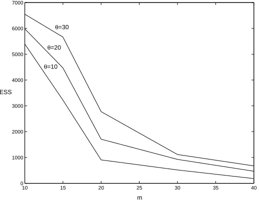
Figure 1: ESS for analysing data sets of size m = 10,15,20,30,40 simulated from the exponentially growing population size model withβ = 0.7 andθ= 10,20,30.
We investigated how the ESS of our method depends on the values of the mutation rate, θ, and the sample size, m. We simulated data from the exponentially growing population size model with rate of exponential growth β = 0.7 and various values of
θ, namely θ= 10,20,30. Figure 1 shows the ESS values for analysing data sets of size
m= 10,15,20,30,40; usingK= 10,000 weighted samples sampled from (3). (Here and below we setφto the value which minimises the likelihood in Eq. 5; though results are insensitive to this choice.) It can be seen that the ESS decreases with m, but increases with θ. The results suggest that for θ = 10 analysing sample sizes of up to 20–40 is reasonable, with slightly larger sample sizes possible for the larger θ values. The speed of this approach means that analysis for larger values ofm should be possible by increasing K.
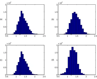
(a) The constant population size model. For this model λ(t) =t.
(b) The exponentially growing population size model. For this model λ(t) =eβt.
(c) The constant population size followed by exponential growth model. For this model we assume
λ(t) =
se−βt, t < s
se−βs, t≥s .
(d) The bottleneck model. For this model we assume
λ(t) =
1, t < s1 α, s1≤t < s2
2, t≥s2 .
For the analysis below we fixed (a) θ= 15, (b)θ= 15 andβ= 0.7, (c)θ= 15, s= 0.1 and β =−10 log(0.05), and (d) θ= 15, s1 = 0.165, s2 = 0.175 and α = 10. We focus
on inferring the time to the most recent common ancestor (TMRCA); and in particular looking at how robust these inferences are to the specific choice of model.
We simulated K = 10,000 sets of coalescence times from (3), which took under 2 minutes on a desktop PC. Reweighting this sets of times took around 1 second for each model. The resulting Histograms of the samples of the TMRCA for all models are shown in Figure 3, and the respective estimates of the marginal likelihood are (a) 0.4308, (b) 0.6248, (c) 0.0362, and (d) 2.4191×10⁻⁶. The ESS of the weights were between 1,000
and 5,000 for models (a) – (c), and was 98 for (d). The histograms shows that the esimate of the TMRCA appears robust across these different models.
Note that inference for the bottleneck model is more challenging than for the other mod-els as the importance sampling weights depend crucially on the number of coalescences that lie within the period of the bottleneck; and thus can have a large variance (and hence small ESS). The effect of a bottleneck depends primarily on its severity, defined as the product α(s2−s1). Having a bottleneck with similar severity but larger α and
smaller (s2−s1) will lead to a more poorly behaved importance sampler.
Migration Models
0.5 1 1.5 2 2.5 0
0.5 1 1.5
2x 10
4
0.5 1 1.5 2 2.5
0 0.5 1 1.5
2x 10
4
0.5 1 1.5 2 2.5
0 0.5 1 1.5
2x 10
4
(a) (b)
(c) (d)
0.5 1 1.5 2 2.5
0 0.5 1 1.5
2x 10
[image:14.612.155.469.186.441.2]4
Our approach for migration models is based on an approximate likelihood, and firstly we need to check the validity of this approach. To do this we calculated the mean log-likelihood over a set of independent data. The shape of the mean log-likelihood governs the asymptotic behaviour of the method, and in particular for an approximate likelihood method to produce consistent esimates it is required that the mean log-likelihood curve attains its maximum at the true value of the parameters (see Fearnhead, 2003; Smith and Fearnhead, 2005, for further discussion). Thus an important property of an approximate likelihood method is that the mean log-likelihood curve attains its maximum at a value close to the true value.
We simulated 100 coalescent trees with sample size ofm= 10 from the migration model with D = 2 demes, N1 = 3000,N2 = 7000, M12 = 1.2 and M21 = 2.8. The mutation
rate used wasθ= 30. For each data set we based inferences on 2,000 sets of coalescence times simulated from (3), again with φ set to the value that maximises (5). We have estimated the mean log-likelihood at a grid of values ofM12, M21. A contour plot of this
log-likelihood surface is shown in figure 4. The maximum of this curve is indeed close to the true parameter value (maximum atM12= 1.02, M21= 2.52). Similar results are
obtained for a range of migration models (results not shown).
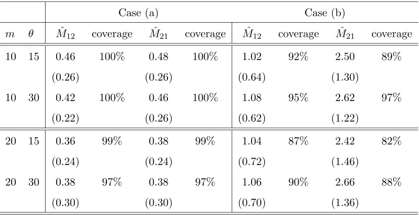
In Table 1 we present results on the performance of our approach, obtained from simu-lated data of size m= 10,20 from the migration model withD= 2 demes for different values of the model parameters. We consider 2 sets of parameters; (a)N1=N2 = 5000, M12 = M21 = 0.4, and (b) N1 = 3000, N2 = 7000, M12 = 1.2, M21 = 2.8. In each
case we report the average of the most likely parameter values across 100 data sets, the standard errors of these estimates (in parentheses) and the associated coverage of the 95% likelihood-based confidence intervals (CIs). The average CPU cost of analysing a data set on a laptop PC is 30sec for the m= 10 case and 50sec for them= 20 case.
For comparison we reanalysed them= 10, M12=M21= 0.4 data sets usinggenetree
0.4 0.8 1.2 1.6 2.0 2.4 2.8 3.2 3.6 4.0 0.2
0.4 0.6 0.8 1.0 1.2 1.4 1.6 1.8 2.0
M21 M
[image:16.612.171.451.26.253.2]12
Figure 4: Contour plot of the mean log-likelihood surface ofM12, M21obtained from 100
simulated coalescent trees under the migration model withD= 2 demes (each contour corresponds to 0.05 units of log-likelihood). The true parameter values are M12 = 1.2
and M21= 2.8.
Case (a) Case (b)
m θ Mˆ12 coverage Mˆ21 coverage Mˆ12 coverage Mˆ21 coverage
10 15 0.46 100% 0.48 100% 1.02 92% 2.50 89%
(0.26) (0.26) (0.64) (1.30)
10 30 0.42 100% 0.46 100% 1.08 95% 2.62 97%
(0.22) (0.26) (0.62) (1.22)
20 15 0.36 99% 0.38 99% 1.04 87% 2.42 82%
(0.24) (0.24) (0.72) (1.46)
20 30 0.38 97% 0.38 97% 1.06 90% 2.66 88%
(0.30) (0.30) (0.70) (1.36)
Table 1: Performance of our approximate likelihood approach for simulated data under the migration model with D = 2 demes for different scenarios; (a) N1 = N2 = 5000, M12=M21= 0.4, and (b) N1 = 3000, N2 = 7000,M12 = 1.2,M21= 2.8. In each case
[image:16.612.107.521.380.593.2]100 simulations (in comparison with an ESS of>1,000 for our method). The estimates from the two methods were highly correlated (correlation co-efficient 0.77). The root mean square error of our estimates was about 10% higher than that of genetree. This maybe due to the extra statistical efficiency of the true mle, or it be partly due to our choice of driving value (see discussion of Fearnhead and Donnelly, 2001); and rerunning
genetreewith a driving value that is away from the truth (1.0 as opposed to 0.4) gives estimates with root mean square error that is 30% greater than our estimates.
Continuous Spatial Models
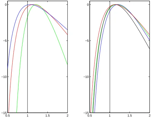
Finally we present results for the continuous spatial models. Again here we can only estimate the parameters of the spatial model relative to the mutation rate θ. There-fore, we fix the parameters of the demographic model to their true values and look at estimates of the spatial parameters.
Firstly we check the validity of the approximate likelihood through calculating the mean log-likelihood for a range of parameters. For each set of parameters we simulated 100 data sets and then used our approximate approach withK= 5000 to estimate the like-lihood curve ofσ, the parameter governing the rate of spatial dispersion, and to obtain samples from the posterior distribution of the location of the MRCA. Combining infor-mation from all of the 100 simulated trees we have estimated the average log-likelihood at a grid of values of σ. Figure 5 shows the resulting mean log-likelihood curves for a range of values of the sample size, m, the mutation rate, θ, and the population growth parameter, β. In each caseσ= 1. The accuracy of the method appears to be primarily dependent on m; with the asymptotic bias of the method increasing as mincreases (as the value ofσ for which the maximum of the mean log-likelihood curve is attained gets further away from σ = 1 as m increases). For values of m up to 10 this bias appears small.
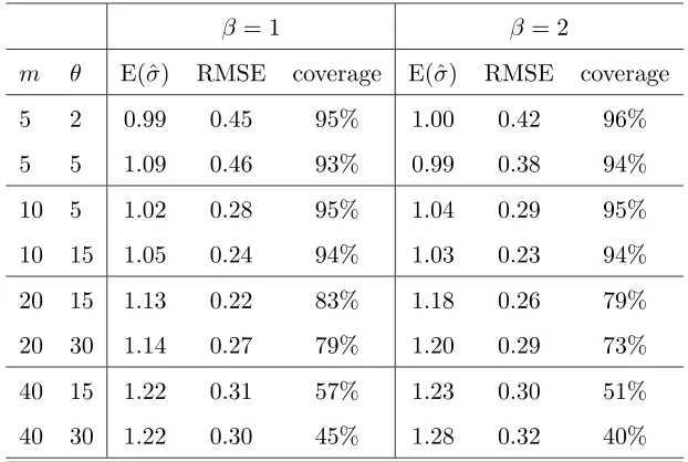
In Table 2 we present a summary of the estimates ofσ across the 100 data sets for each set of parameter values; and in Table 3 we give the mean square error of the estimate of the position of the MRCA (these estimates had negligible bias); due to symmetry we show only the mean square error for esimating one co-ordinate of the position.
We see that the estimates of σ are accurate for values of m up to 10; beyond this we notice a bias in our estimates, and the root mean square error actually increases when we move from m= 10 to m = 40. Coverage properties also appear good for values of
0.5 1 1.5 2 −15
−10 −5 0
0.5 1 1.5 2 −15
[image:18.612.181.441.16.223.2]−10 −5 0
Figure 5: Plots of the log-likelihood surface of σ for a range of parameter values, each obtained from 100 simulated data sets. Left-hand plot: θ = 15, β = 1 and m = 10 (blue) m = 20 (red) and m = 40 (green); right-hand plot: m= 20 and θ = 30, β = 1 (black), θ= 30,β = 2 (blue), θ= 15, β = 1 (red), andθ= 15, β = 2 (green).
The values ofβ and θappear to have had little effect on the results. These results are consistent with those from Figure 5, with the bias of the estimator starting to dominate its performance for m= 20 and particularlym= 40.
For comparison with our estimate of the position of the MRCA, we also calculated a simple unbiased estimate for each data set which is obtained by taking the average of the locations of the sample. The mean square error of one co-ordinate of the position is also shown in Table 3. Our approach is uniformly more accurate - with quite noticeable reduction in mean square error for m = 20 and m = 40. Note that the estimates are more accurate for β = 2 due to the tree being shorter, and thus the spatial spread of the data less, than forβ = 1.
To demonstrate the advantage of post-processing a sample of genealogical trees, rather than conditional analysis based on a single tree, we considered the alternative approach of inferring σ given a single estimate of the genelogy. Such an approach (i) obtains an estimate of the coalescent times ˆt; and (ii) bases inference on the conditional likelihood
p(x|ˆt, σ). We used the maximum likelihood estimator of ˆt(which for these models can be calculated using the method of Meligkotsidou and Fearnhead, 2005).
obtained for larger values of m. One difficulty with using the maximum likelihood esimate oftis that this is 0 for identical sequences, which leads to an invalid conditional likelihood (p(x|ˆt, σ) =0, for allxandσ). Thus in our analysis below we simulate data conditional on a sample having no identical sequences.
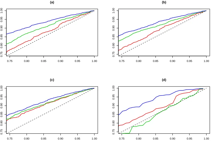
Figure 6 gives Probability-Probalitiy (PP) plots of the Likelihood Ratio statistics for testingσ = 1 against draws from a chi-squared distribution with one degree of freedom. We show this plot as this PP plot is related to the coverage properties of confidence intervals for the parameter, and if the Likelihood Ratio statistic is approximately dis-tributed as a chi-squared distribution with one degree of freedom, then it shows that the likelihood method is correctly quantifying the uncertainty in the parameter. This analysis is slightly complicated for the m= 2 case, as the sample size is too small for the asymptotic limit of the Likelihood ratio statistic to be a very good approximation -thus we also show the PP plot for the Likelihood Ratio statistic conditional on knowing the true coalescence time. For each value of θ we give PP plots for the new approx-imate likelihood method, the conditional analysis for the data sets with at least one segregating site. For smaller values of θ the approach that conditions on the mle for the coalescence time substantially under-estimates the uncertainty of the estimate for
σ. As θ increases the distribution of the LR statistics approaches the distribution of the LR statistic for the likelihood of σ conditional on the true value of the coalescence time.
The effect of conditioning on the mle of the times is less pronounced on the point estimates ofσ. For them= 5 case, the two sets of mles are highly correlated (correlation 0.96), and give almost identical root mean square error, though conditioning on the mle appears to give slight underestimates ofσ. A measure of the efficiency of this approach can be seen by looking at the correlation of the esimates from our method with those conditional on the true coalescence times, this again is high (correlation 0.80).
DISCUSSION
chang-β= 1 β = 2
m θ E(ˆσ) RMSE coverage E(ˆσ) RMSE coverage
5 2 0.99 0.45 95% 1.00 0.42 96%
5 5 1.09 0.46 93% 0.99 0.38 94%
10 5 1.02 0.28 95% 1.04 0.29 95%
10 15 1.05 0.24 94% 1.03 0.23 94%
20 15 1.13 0.22 83% 1.18 0.26 79%
20 30 1.14 0.27 79% 1.20 0.29 73%
40 15 1.22 0.31 57% 1.23 0.30 51%
[image:20.612.157.468.37.246.2]40 30 1.22 0.30 45% 1.28 0.32 40%
Table 2: Performance of our conditional likelihood approach at estimating σ for the spatial model. We report the mean of the estimates of σ (truth σ = 1), the root mean square error of the estimates, and the coverage probability of 95% approximate confidence intervals. (The grid ofσ values ranged from 0–4 form= 5 andm= 10; and 0–2 form >10.)
β = 1 β = 2
m θ CL SM CL SM
5 2 0.39 0.53 0.23 0.27 5 5 0.29 0.39 0.26 0.31 10 5 0.45 0. 49 0.26 0.28 10 15 0.43 0.44 0.30 0.31 20 15 0.37 0.44 0.27 0.34 20 30 0.31 0.38 0.27 0.35 40 15 0.44 0.48 0.21 0.26 40 30 0.46 0.51 0.30 0.39
0.75 0.80 0.85 0.90 0.95 1.00
0.75
0.80
0.85
0.90
0.95
1.00
(a)
0.75 0.80 0.85 0.90 0.95 1.00
0.75
0.80
0.85
0.90
0.95
1.00
(b)
0.75 0.80 0.85 0.90 0.95 1.00
0.75
0.80
0.85
0.90
0.95
1.00
(c)
0.75 0.80 0.85 0.90 0.95 1.00
0.75
0.80
0.85
0.90
0.95
1.00
[image:21.612.138.490.165.404.2](d)
ing the method of simulating the data will only affect step (B) of the algorithm, with the denominator of the importance sampling weights being the prior of the model un-der which the sample of genealogies was generated.) All that is required is that the there is computational machinery (e.g. MCMC algorithms) that can produce samples of genealogies for the data. For example, analysis of more general mutation models is possible using the Bayesian phylogenetic packages such as MrBayes (Ronquist and Hulsenbeck, 2000) andBambe(Larget and Simon, 1999), while analysis of(recombining) bacterial MLST data is possible using ClonalFrame (Didelot and Falush, 2006).
We first considered inference for a variable population size, and robustness of inference of coalescence times to changes in the model for the population size. An importance sampling approach, which is “exact” in the limit as the computational cost increases, is possible here. In practice the efficiency of this method will depend on the sample size and the mutation rate; efficiency decreasing as sample size increases or mutation rate decreases. Our results suggest that this approach is practicable for sample sizes of up to 50 chromosomes. The advantage of this post-processing is that it enables a data set to be analysed quickly under a range of different models. As such we view that this approach will be useful in terms of a preliminary analysis of a potentially large data set. We can first subsample an appropriate number of chromosomes (of the order of 10–50), and analyse these under a variety of models. This will help inform us as to what are the appropriate models for analysing the complete data (using a more dedicated/computationally-intensive approach), and also give insights as to how robust the results about the coalescence times of the tree will be.
of the genealogy will converge to a point mass on the true genealogy). In practice we observe the approximate likelihood method performs well for relatively small sample sizes (up to 20 chromosomes). For larger sample sizes, the genealogical prior we use is not correctly capturing the distribution of some of the coalescence times, and this then starts to introduce biases into the method.
However, our method can be applied to large data using a composite likelihood ap-proach. A large data set can be split into smaller subsamples (with the possibility of each chromosome appearing in many subsamples); the approximate log-likelihood calculated for each subsample; and these approximate log-likelihood curves combined through adding them together. An estimate of the parameter(s) is given by the value(s) that maximise this composite log-likelihood. The performance of such a method is governed by the shape of the mean of the log of the approximate likelihood, such as shown in Figures 5 (see Fearnhead, 2003). And these results suggest that the methods should perform well is the composite likelihood is based upon analysisng subsamples of relatively small size (with m up to 10).
In particular a pairwise likelihood approach is likely to be a simple method for analysing continuous spatial data sets (currently there are few methods for analysing such models). For such a pairwise approach it is simple to allow for quite general models of the spatial spread of the population through time, all that is required is the specification of a family of densities,p(x1, x2;t), for the probability of two chromosomes which share a common
References
Bahlo, M. and Griffiths, R. C. (1998). Inference from gene trees in a subdivided popu-lation.Theoretical Population Biology 57, 79–95.
Beerli, P. and Felsenstein, J. (1999). Maximum-likelihood estimation of migration rates and effective population numbers in two populations using a coalescent approach.
Genetics 152, 763–773.
Brooks, S. P., Manopoulou, I. and Emerson, B. C. (2007). Bayesian Statistics 8, chap-ter Assessing the affect of genetic mutation: A Bayesian framework for dechap-termining population history from DNA sequence data. Oxford University Press, Oxford.
Coop, G. and Griffiths, R. C. (2004). Ancestral inference on gene trees under selection.
Theoretical Population Biology 66, 219–232.
Didelot, X. and Falush, D. (2006). Inference of bacterial microevolution using multilocus sequence data.submitted .
Drummond, A. J., Rambaut, A., Shapiro, B. and Pybus, O. G. (2005). Bayesian co-alescent inference of past population dynamics from molecular sequences.Molecular Biology and Evolution 22, 1185–1192.
Emerson, B. C. and Hewitt, G. M. (2005). Phylogeography. Current Biology 15, 367– 371.
Fearnhead, P. (2003). Consistency of estimators of the population-scaled recombination rate.Theoretical Population Biology 64, 67–79.
Fearnhead, P. and Donnelly, P. (2001). Estimating recombination rates from population genetic data.Genetics 159, 1299–1318.
Fearnhead, P. and Donnelly, P. (2002). Approximate likelihood methods for estimating local recombination rates (with discussion). Journal of the Royal Statistical Society, series B 64, 657–680.
Fearnhead, P. and Meligkotsidou, L. (2004). Exact filtering for partially-observed continuous-time Markov models. Journal of the Royal Statistical Society, series B
66, 771–789.
Felsenstein, J. (1981). Evolutionary trees from DNA sequences: a maximum likelihood approach. Journal of Molecular Evolution 17, 368–376.
French, N. P., Barrigas, M., Brown, P., Ribiero, P., Williams, N. J., Leatherbarrow, H., Birtles, R., Bolton, E., Fearnhead, P. and Fox, A. (2005). Spatial epidemiology and natural population structure of campylobacter jejuni colonising a farmland ecosystem.
Environmental Microbiology 7, 1116–1126.
Griffiths, R. C. and Marjoram, P. (1996). Ancestral inference from samples of DNA sequences with recombination.Journal of Computational Biology 3, 479–502.
Griffiths, R. C. and Tavar´e, S. (1994a). Sampling theory for neutral alleles in a varying environment. Philosophical Transactions of the Royal Society of London. Series B
344, 403–410.
Griffiths, R. C. and Tavar´e, S. (1994b). Simulating probability distributions in the coalescent.Theoretical Population Biology 46, 131–159.
Kuhner, M. K., Yamato, J. and Felsenstein, J. (1998). Maximum likelihood estimation of population growth rates based on the coalescent.Genetics 149, 429–434.
Kuhner, M. K., Yamato, J. and Felsenstein, J. (2000). Maximum likelihood estimation of recombination rates from population data.Genetics 156, 1393–1401.
Larget, B. and Simon, D. L. (1999). Markov chain Monte Carlo algorithms for the Bayesian analysis of phylogenetic trees. Molecular Biology and Evolution 16, 750– 759.
Liu, J. S. (1996). Metropolised independent sampling with comparisons to rejection sampling and importance sampling.Statistics and Computing 6, 113–119.
Meligkotsidou, L. and Fearnhead, P. (2005). Maximum likelihood estimation of coales-cence times in genealogical trees.Genetics 171, to appear.
Rannala, B. and Yang, Z. (1996). Probability distribution of molecular evolutionary trees: A new method of phylogenetic inference.Journal of Molecular Evolution 43, 304–311.
Rue, H. and Held, L. (2005). Gaussian Markov Random Fields: Theory and Applica-tions. CRC Press/Chapman and Hall.
Shen, P., Wang, F., Underhill, P. A., Franco, C., Yang, W., Roxas, A., Sung, R., Lin, A. A., Hyman, R. W., Vollrath, D., Davis, R. W., Carvalli-Sforza, L. and Oefner, P. J. (2000). Population genetic implications from sequence variation in four Y chromosome genes.Proceedings of the National Academy of Science 97, 7354–7359.
Smith, N. G. C. and Fearnhead, P. (2005). A comparison of three estimators of the population-scaled recombination rate: accuracy and robustness.Genetics171, 2051– 62.
Stephens, M. and Donnelly, P. (2000). Inference in molecular population genetics (with discussion).Journal of the Royal Statistical Society, Series B 62, 605–655.
Templeton, A. R., Boerwinkle, E. and Sing, C. F. (1987). A Cladistic Analysis of Phenotypic Associations With Haplotypes Inferred From Restriction Endonuclease Mapping. I. Basic Theory and an Analysis of Alcohol Dehydrogenase Activity in Drosophila.Genetics 117, 343–351.
Underhill, P. A., Passarino, G., Lin, A. A., Shen, P., Lahr, M., Foley, R. A., Oefner, P. J. and Cavalli-Sforza, L. L. (2001). The phylogeography of Y chromosome binary haplotypes and the origins of modern human populations.Annals of Human Genetics
65, 43–62.
Wilkins, J. F. (2004). A separation-of-timescales approach to the coalescent in a con-tinuous population.Genetics 168, 2227–2244.
Wilkins, J. F. and Wakeley, J. (2002). The coalescent in a continuous, finite, linear population.Genetics 161, 873–888.
APPENDIX
The prior (2) can be obtained by simulating s from the prior with φ = 1, and then letting t =φs. Thus if we define S and sijs to satisfy T =φS and tij =φsij, so they
are the respective times obtained froms, we get that
Cov(Xi, Xj) =σ2φ(S−sij).
Thus the intuition behind the result is that, as under the prior the data is solely infor-mative about the product σ2φ, using the scale invariance prior for φ will result in no information about σ.
Formally we use the fact that
p(x|σ) = Z Z
p(x|σ, φ,s)p(φ)dφp(s)ds.
We consider the integral with respect to φ, assuming a given s, and demonstrate that this does not depend onσ, from which the fact thatp(x|σ) does not depend onσfollows. For notational simplicity we assume µ= 0 in the following.
Now for our given s let Σ be the covariance matrix obtained when σ = φ = 1, so Σij = (S−sij) for i, j= 1, . . . , m. Further letQ= Σ−1 andA=xTQx/2. Then
Z
p(x|σ, φ,s)p(φ)dφ
∝
Z
(σ2φ)−m/2exp{−A/(σ2φ)}φ−1dφ.
= σ−mZ γm/2−1exp{−γA/(σ2)}dγ
= σ−mΓ(m/2)(A/σ2)−m/2.