Munich Personal RePEc Archive
Optimal operational monetary policy
rules in an endogenous growth model: a
calibrated analysis
Arato, Hiroki
Graduate School of Economics, Kyoto University, Japan Society for
the Promotion of Science
May 2008
Online at
https://mpra.ub.uni-muenchen.de/8547/
Optimal operational monetary policy rules in
an endogenous growth model: a calibrated
analysis
∗
Hiroki Arato
†May 2008
abstract
We construct an endogenous growth model with new Keynesian-type sticky prices and wages. In this model, monetary policy affects long-run output growth. We characterize the optimal operational monetary policy rule in this economy. We find that even though stabi-lization of output growth increases long-run output growth, the opti-mal monetary policy rule is the rule that makes interest rate respond to price and wage actively and output growth mutely, similar as in exogenous growth models. We also find that the optimal monetary policy rule virtually maximizes mean growth. These results suggest that although long-run growth is important for welfare, new Keyne-sian’s claim that monetary policy should stabilize nominal variables is highly robust.
Keywords: Monetary policy, Sticky price and wage, Business cycle fluctuations, Productivity growth
JEL classification: E31, E32, E52, O41
∗I appreciate many helpful comments and suggestions received from my adviser
To-moyuki Nakajima. I am also grateful to Takayasu Matsuoka and workshop participants at Osaka University. Any remaining errors are the sole responsibility of my own. This study is financially supported by the research fellowships of the Japan Society for the Promotion of Science for young scientists.
†Japan Society for the Promotion of Science and Graduate School of Economics, Kyoto
1
Introduction
Our aim in this paper is to give some answers to the following questions. How much does monetary policy affect long-run growth? Does the long-run growth effect change the features of the optimal monetary stabilization policy rule? In order to highlight the growth and welfare effect of monetary policy, we incorporate Calvo (1983)-type sticky prices and wages to the two-capital convex model of endogenous growth. We here consider two types of growth effects, that is, the growth effect caused by the changes of long-run target rate of inflation under the deterministic environment and the effect arisen from uncertainty and monetary stabilization policy rules such as the Taylor rule. We shall call the former the deterministic growth effect and the latter
the stochastic growth effect. Our motivations and findings of this research are as follows.
We first explain the deterministic growth effect. Empirical studies using cross-country data claim that long-run growth and inflation have a negative relationship. Calibrating the model, we find that in steady state, price sticki-ness cause negative long-run relationship between growth and inflation under positive inflation rate and that the magnitude of this relationship strongly depends on the degree of price stickiness. In the existence of price stickiness, non-zero inflation is a source of distortion which comes from price dispersion This distortion reduces resources which can be used for investment and so decreases output growth. This finding suggests that the various strength of price stickiness account for the difference of the relationship across countries. Second, for the stochastic growth effect, Jones et al. (2005b) show that this type of model has the effect of uncertainty on long-run growth. Incor-porating nominal rigidities into their model can cause changes of long-run growth rate through changes of interest rate policy rules. Moreover, It is also known that this class of model improves over simple (exogenous growth) RBC models.1 Hence, the endogenous growth models with nominal
rigidi-ties has the potential abilirigidi-ties accounting the business cycle properrigidi-ties better than existing New Keynesian models. The relationship between fluctuations and growth is also important from normative perspective. In his seminal work, Lucas (1987) shows that the cost of business cycles is much less than that of growth. It is well known that his claim is strongly robust,2 but it
does not imply that fluctuations are negligible for the macroeconomics at all, because even if fluctuations itself has the small welfare effect, fluctuations can affect the long-run growth through the optimization of the economic
1See Jones et al. (2005a). Comin and Gertler (2006) also show that other endogenous
growth model accounts for the medium term properties of business cycles well.
agents(Barlevy, 2004b).
For these reasons, endogenizing productivity growth can be thought to be important for the analysis of business cycle and stabilization policy. Most of studies about short-run monetary policy (New Keynesian approach), how-ever, have been ignored the effect of monetary policy on long-run economic growth. We conjecture that the reason is purely technical issue. In most of New Keynesian studies, they approximate to the policy functions around non-stochastic steady-state up to first-order. In linear models, unconditional mean of endogenous variables are idendical to the non-stochastic steady-state value. Hence, even if long-run growth rate is endogenous, higher-order ap-proximation is needed for the model to show the growth effect. We apply the numerical computation method which approximating to the policy function up to second-order developed by Schmitt-Grohe and Uribe (2004). Their nu-merical method enables us to address the relationship between stabilization policy and long-run growth because endogenous growth models with nominal rigidities approximated up to second-order do not hold certainty equivalence so that long-run growth rate is no longer identical to non-stochastic steady-state growth rate.
Solving our model by second-order approximation, we obtain some find-ings about the stochastic growth effect and about the optimal operational monetary policy as follows. First, in our model with stochastic disturbances, the long-run rate of output growth is affected by the monetary stabiliza-tion policy rules, especially policy rule responding to output though, under simple Taylor rule, deviation of annual growth rate from deterministic bal-anced growth path is very small, about −10−3
relationship between the optimal monetary stabilization policy and long-run growth. They show analytically that optimal monetary policy is identical to the growth-maximizing policy in the endogenous growth model with neo-classical-type nominal wage rigidity.
This paper is organized as follows. In the next section, we present the model into which stochastic endogenous growth and nominal rigidities are fused, and calibrate the model. Section 3 analyzes the steady state and shows some results about the deterministic growth effect. Section 4 consider the stochastic growth and welfare effect under versions of Taylor rule. Section 5 considers the optimal operational interest-rate feedback rule. Section 6 concludes this paper.
2
The model
The model is a two-capital convex model of endogenous growth by Jones et al. (2005a) incorporating Calvo-type sticky prices and wages, physical and human capital investment adjustment costs, and habit persistence.
2.1
Households
The representative families, across whose menbers consumption and hour worked are identical, have preferences which are described by the following utility function,
E0
∞
∑
t=0
βtU(Ct−bCt−1,1−nt),
with
U(Ct−bCt−1,1−nt)≡
{ (C
t−bCt−1)1−σ(1−nt)ψ(1−σ)
1−σ whenσ6= 1
log(Ct−bCt−1) +ψlog(1−nt) whenσ = 1,
where Et is the standard expectations operator conditional on information
at time t,Ct denotes per capita consumption, nt represents per capita labor
Dixit-Stiglitz aggregator. Hence the demand for Yit is given by
Yit =
(
Pit
Pt
)−θ
Yt,
Yt=Ct+ItK+ItH (1)
and price index Pt is
Pt=
(∫ 1
0 P1−θ
it di
)1−1θ
, (2)
whereYt is aggregate absorption,Pit denotes the price of goodi, andItK and
IH
t represent physical and human capital investment per capita, respectively.
Households’ expenditures on consumption goods are subject to a cash-in-advance constraint
Mth ≥νhCt, (3)
where Mh
t denotes real money balances holding by households in period t
and νh is a parameter.
Households own human capital Ht, and physical capital Kt. Capital
accmulation equations are assumed as follows.
Kt+1 = (1−δK)Kt+ItK−
aK
2
(
IK t
IK t−1
−ηFK
)2
ItK (4)
Ht+1 = (1−δH)Ht+ItH −
aH
2
(
IH t
IH t−1
−ηHF
)2
ItH (5)
where δK and δH denote the depreciation rates with respect to physical and
human capital, and aK and aH represent the investment adjustment cost
parameters for physical and human capital,3 respectively.
Following Schmitt-Grohe and Uribe (2005) (henceforth SGU), labor sup-ply is decided by “a union”, which supplies labor monopolistically to a con-tinuum of labor markets indexed by j ∈ [0,1]. As we shall see below, the demand for labor in the labor market j is
njt =
(
Wjt
Wt
)−θ˜
ndt. (6)
3This type of investment adjustment cost function is assumed in Christiano et al.
and nominal wage index is
Wt =
(∫ 1
0
W1−θ˜
jt dj
)11 −θ˜
(7)
where nd
t is the aggregate labor demand and Wjt denotes the nominal wage
rate in the labor market j. We define real wage index, wt ≡ Wt/Pt, and
real wage rate in labor market j, wjt ≡ Wjt/Pt, respectively. The resource
constraint of labor supply is
nt=
∫ 1
0
njtdj, (8)
From (7) and (8), a resource constraint which the union faces is obtained as
nt=ndt
∫ 1
0
(
wjt
wt
)−θ˜
dj. (9)
We assume that households can access to a complete set of nominal state-contingent claims and that the effective labor is defined as product of hour worked and human capital, so that households’ intertemporal budget con-straint is
Etdt,t+1 Xt+1
Pt
+Mth+Ct+ItK+ (1 +τh)ItH
= Xt Pt
+Pt−1
Pt
Mth−1+ (1 +τ
h)
∫ 1
0
(
wtj
wt
)−θ˜
ndtHtwtjdj +rtKKt+ Φt+Tt,
(10)
where dt,s is nominal stochastic discount factor, Xt is nominal payment in
periodt,rK
t denotes real rental rate on physical capital, Φtis profits received
from firms, and Tt denotes the transfer from the government. τh represents
human capital investment tax rate and wage subsidy rate to eliminate dis-tortion which comes from monopolistic competition in labor markets. We assume τh = 1/(˜θ−1).
We assume wage stickiness following Calvo (1983) and SGU, that is, in each period the union cannot reoptimize the nominal wage in a fraction ξw ∈[0,1) of randomly chosen labor markets. Following SGU, in these
non-optimized markets, the nominal wages are (fully or partially) indexed to the nominal good-price inflation in the previous period.4 Therefore, the nominal 4In some models where labor productivity grows exogenously such as SGU, the nominal
wage setting rule is
Wjt =
{
˜
Wt if the wage can be re-optimized,
πχt˜−1Wj,t−1 otherwise,
where ˜Wt is the optimal nominal wage rate in period t, πt ≡ Pt/Pt−1 is
nominal good-price inflation rate. Defining the optimal real wage rate as ˜
wt≡W˜t/Pt, We can rewrite the rule as
wjt =
{
˜
wt if the wage can be re-optimized, πtχ˜−1
πt wj,t−1 otherwise.
(11)
Households maximize (2.1) subject to (3), (4), (5), (9), (10), the sticky wage assumption (11), and the no-Ponzi game condition, choosing processes forCt,nt,Xt+1,Mt,ItK,ItH,Kt+1,Ht+1, and wtj. Let us define the Lagrange
multipliers associated with (3), (4), (5), (9), (10) as βtΛ
tζt, βtΛtqKt , βt(1 +
τh)Λ tqtH, β
tΛ twtHt
˜
µt , and β
tΛ
t respectively. Restricting our attention to the
strictly-positive nominal interest rate equilibria, we obtain the first-order conditions with respect to Ct, nt, Xt+1, Mt, ItK, ItH, Kt+1, Ht+1 as follows.
Ct : Λt(1 +νfζt) = (Ct−bCt−1) −σ
(1−nt)ψ(1
−σ)
−βbEt(Ct+1−bCt)
−σ
(1−nt+1)ψ(1
−σ)
,
(12)
nt :
ΛtwtHt
˜ µt
=ψ(Ct−bCt−1)
1−σ
(1−nt)ψ(1−σ)−1, (13)
Xt+1 : dt,t+1 =
βΛt+1
Λtπt+1
, (14)
Mt : Λt(1−ζt) =βEt
Λt+1 πt+1
, (15)
ItK : Λt= ΛtqtK
[
1− a F K 2 ( IK t IK t−1
−ηKF
)2
−aFK
(
IK t
IK t−1
−ηFK
)
IK t
IK t−1
]
+βEtΛt+1qtK+1aFK
(
IK t+1 IK
t
−ηKF
) ( IK t+1 IK t )2 , (16)
ItH : Λt= ΛtqtH
[
1− a F H 2 ( IH t IH t−1
−ηFH
)2
−aFH
(
IH t
IH t−1
−ηHF
)
IH t
IH t−1
]
+βEtΛt+1qtH+1aFH
(
IH t+1 IH
t
−ηHF
) ( IH t+1 IH t )2 , (17)
Kt+1 : ΛtqtK =βEtΛt+1[rtK+1+qtK+1(1−δK)], (18)
From (14) and the definition of nominal interest rate, 1/Rt=Etdt,t+1, we
obtain the well-known fisher relationship, 1
Rt
=βEt
Λt+1
Λtπt+1
. (20)
and, from (15) and (20), the cost of holding money ζt is representing that
ζt= 1−R
−1
t . (21)
Next, we consider optimal wage setting behavior. The parts of Lagrangian that are relevant for wage setting is
Lw t =Et
∞
∑
s=0
(βξw)s
[
(1 +τh)Λ
t+sndt+sHt+sw˜tX˜t,t+s
(w˜tX˜t,t+s
wt+s
)−θ˜
−Λt+swt+sHt+s
˜ µt+s
ndt+s(w˜tX˜t,t+s wt+s
)−θ˜]
,
where,
˜ Xt,t+s=
{
1 s= 0,
πχt˜
πt+1 · · · · · πχt˜+s−1
πt+s s= 1,2,· · · . The first-order conditions with respect to ˜wt is
Et
∞
∑
s=0
(βξw)sΛt+sndt+sHt+s
(
˜ wt
wt+s
)−θ˜
˜ X−θ˜
t,t+s
[
(1 +τh)θ˜−1 ˜ θ w˜t
˜ Xt,t+s−
wt+s
˜ µt+s
]
= 0.
Define F1
t and Ft2 as
Ft1 = (1 +τh)θ˜−1 ˜
θ w˜tEt
∞
∑
s=0
(βξw)sΛt+sndt+sHt+s
(
˜ wt
wt+s
)−θ˜
˜ X1−θ˜
t,t+s,
Ft2 =Et
∞
∑
s=0
(βξw)sΛt+sndt+sHt+s
(
˜ wt
wt+s
)−θ˜
˜ X−θ˜
t,t+s
wt+s
˜ µt+s
,
respectively, and we obtain the recursive formulation of optimal wage setting behavior,
Ft1 = (1 +τh)θ˜−1 ˜ θ Λtn
d tHt
(
˜ wt
wt
)−θ˜
˜
wt+βξwEt
(
˜ wt
˜ wt+1
)1−θ˜(
πχt˜
πt+1
)1−θ˜
Ft1+1,
(22)
Ft2 = ΛtndtHt
(
˜ wt
wt
)−θ˜
wtµ˜
−1
t +βξwEt
(
˜ wt
˜ wt+1
)−θ˜(
πtχ˜ πt+1
)−θ˜
Ft2+1, (23)
2.2
Firms
Each good i is produced by a single firm indexed by i ∈ [0,1] in monopo-listically competitive good market. The production technology of Firm i is represented by the following Cobb-Douglas production function,
Yit=AtKitαZ1
−α
it ,
where At represents exogenous aggregate productivity, Kit and Zit denotes
physical capital and the effective labor demanded by firm i, respectively. We impose a cash-in-advance constraint for wage payments
Mitf =νfwtZit, (25)
where Mitf denotes the demand for real money balances by firm i and νf is
a parameter. The cost of holding money is (1−R−1
t )M f
it, hence the nominal
total production cost of firm i is represented as
rtKKit+wtZit+ (1−R
−1
t )M f it.
The first-order conditions of the cost minimization problem are given by
rtK =αAtKα
−1
it Z1
−α
it mct, (26)
wt[1 +νf(1−R
−1
t )] = (1−α)AtKitαZ
−α
it mct, (27)
(
Pit
Pt
)−θ
Yt =AtKitαZ1
−α
it , (28)
where mct represents real marginal cost. Note that the real marginal cost is
in common among the firms, hence the subscript representing the firm index i is dropped.
We assume price stickiness following Calvo (1983) and Yun (1996), that is, each period a fractionξp ∈[0,1) of randomly chosen firms cannot reoptimize
the nominal price of their producted good. Formally, the firms set their nominal prices according to the following rule,
Pit=
{
˜
Pt if the firm can set their price optimally,
πtχ−1Pi,t−1 otherwise.
(29)
Hence, profit maximization problem are formulated as
max Et
∞
∑
s=0
dt,t+sPt+sξsp
(1 +τY) (
Xt,t+sP˜t
Pt+s
)1−θ
Yt+s−
(
Xt,t+sP˜t
Pt+s
)−θ
Yt+smct+s
where,
Xt,t+s =
{
1 s= 0,
πχt · · · · ·πtχ+s−1 s= 1,2,· · · ,
and where τY = 1/(θ−1) represents production subsidy rate to eliminate
distortion which comes from monopolistic competition in good markets. The first-order condition with respect to ˜Pt is
Et
∞
∑
s=0
dt,t+sξspYt+s
(1 +τY)(θ−1)X1
−θ
t,t+s
(
˜ Pt
Pt+s
)−θ
−θX−θ
t,t+s
(
˜ Pt
Pt+s
)−θ−1
mct+s
= 0.
Define X1
t and Xt2 as
Xt1 ≡Et
∞
∑
s=0
dt,t+sξpsYt+sXt,t−θ+s
(
˜ Pt
Pt+s
)−θ−1
mct+s,
Xt2 ≡Et
∞
∑
s=0
dt,t+sξpsYt+sX1
−θ
t,t+s
(
˜ Pt
Pt+s
)−θ
,
respectively, and we obtain the recursive formulation of optimal price setting behavior,
Xt1 = ˜p−θ−1
t Ytmct+ξpEtdt,t+1(πχt)
−θ
(
˜ pt
πt+1p˜t+1
)−θ−1
Xt1+1, (30)
Xt2 = ˜p−θ
t Yt+ξpEtdt,t+1(πtχ)1
−θ
(
˜ pt
πt+1p˜t+1
)−θ
Xt2+1, (31)
θXt1 = (1 +τY)(θ−1)Xt2, (32)
where we define ˜pt ≡P˜t/Pt.
Finally, we show that labor demand in the market j and nominal wage index are described as the form of (6) and (7), respectively. The effective labor input of firm i, Zit, is assumed to be a composite effective labor made
by the following aggregator
Zit=
[∫ 1
0
(Zitj)θ˜−θ˜1dj
]
˜
θ
˜
θ−1
,
assumed to be identical across the family menbers. More formally, Zitj ≡
njitHt, where njit represents the labor demand by firm i in labor market j.
Hence, the “composite labor” demand by firm i, nit, can be described as
nit=
[∫ 1
0
(njit)θ˜−θ˜1dj
]
˜
θ
˜
θ−1
,
and
Zit=nitHt, (33)
that is, the composite effective labor input can be written as the product of the composit labor and human capital.
The cost minimization problem of firm iwith respect to labor is
min
∫ 1
0
Wjtnjitdj
s.t.nit =
[∫ 1
0
(njit)θ˜−θ˜1dj
]
˜
θ
˜
θ−1
.
Define the Lagrange multiplier as Wt, which represents nominal wage index
because it is marginal cost of composite labor, and we obtain the following equations
njit =
(
Wjt
Wt
)−θ˜
nit (34)
Wt=
[∫ 1
0
(Wjt)1
−θ˜
dj
]1−1θ˜
(35)
The equation (35) is identical to the equation (7). By defining aggregate labor demand in market j and aggregate composite labor demand as
njt ≡
∫ 1
0 njitdi
and
ndt ≡
∫ 1
0
nitdi, (36)
respectively. From (34), we obtain the labor demand equation as the form of (6),
njt =
∫ 1
0
njitdi=
∫ 1
0
(
Wjt
Wt
)−θ˜
nitdi=
(
Wjt
Wt
)−θ˜
2.3
Government
Our study focuses only on the monetary policy, hence, for simplicity we assume that the government does not perchase the final good and that all seigniorage is transfered to households. Therefore the intertemporal budget constraint of the government is
(1 +τh)ItH +
(
Mt−
Mt−1
πt
)
=Tt+ (1 +τh)wtndtHt+ (1 +τY)Yt,
where Mt denotes aggregate real money supply. In equilibrium, therefore, it
holds that
Mt =Mth+Mtf =νhCt+νfwtndtHt, (38)
where Mtf ≡
∫1
0 M
f itdi.
Following some rules described below, monetary authority sets the process for the nominal interest rate, Rt.
2.4
Aggregation, Market Clearing, and Exogenous
pro-cess
2.4.1 Price and wage indexes
By equations (2) and (29), we obtain
1 = (1−ξp)˜p1t−θ+ξp
(
πtχ−1
πt
)1−θ
. (39)
By equations (7) and (11), it holds that
w1−θ˜
t = (1−ξw) ˜w1
−θ˜
t +ξw
(
πχt˜−1
πt
)1−θ˜
w1−θ˜
t−1. (40)
2.4.2 Final-good markets
Market clearing condition in good market iis written as
AtKitαZ1
−α
it =
(
Pit
Pt
)−θ
Yt. (41)
By equations (33), (36), the resouce constraint with respect to capital
∫ 1
0
and the fact that, in equilibrium, capital to effective labor ratios are identical across the firms because the firm’s production function is homogeneous of degree one, we can integrate the equation (41) over all good markets. As the result we obtain aggregate resouce constraint
AtKtα(ndtHt)1
−α
=Ytst, (42)
where we define
st≡
∫ 1
0
(
Pit
Pt
)−θ
di,
or as recursive representation,
st= (1−ξp)˜p−tθ+ξp
(
πtχ−1
πt
)−θ
st−1. (43)
st denotes the inefficiency by the price dispersion.
By equations (26), (27), and the fact that, the equilibrium capital to effective labor ratios are identical across the firms, we obtain
rKt =αAtKα
−1
t (ndt)1
−α
H1−α
t mct, (44)
wt[1 +νf(1−R
−1
t )] = (1−α)AtKtα(ndt)
−α
H−α
t mct. (45)
2.4.3 labor markets
By aggregating (37) over all labor markets, we obtain aggregate resouce constraint with respect to labor,
nt =ndts˜t, (46)
where ˜st ≡
∫1
0
(
wjt
wt
)−θ˜
dj denotes the inefficiency by the wage dispersion. We can write the difinition as recursive representation,
˜
st= (1−ξw)
(
˜ wt
wt
)−θ˜
+ξw
(
wt−1
wt
)−θ˜(
πtχ˜−1
πt
)−θ˜
˜
st−1. (47)
2.4.4 Exogenous process
The law of the motion of aggregate productivity At is assumed to be given
by the following exogenous stochastic process
log
(
At
¯ A
)
=ρlog
(
At−1
¯ A
)
+σǫǫt, (48)
0≤ρ <1, ǫt∼N(0,1),
2.5
Stationary Competitive Equilibrium
In the environment described above, some of endogenous variables are not stationary along the balanced-growth path because the economy shows en-dogenous growth by the same mechanism as Jones et al. (2005b).5 We
there-fore rewrite these variables to be stationary. For this purpose, we categorize the nonstationary variables into three groups and divide these variables in each group by the appropriate factors. The first group are composed of Ct,
Yt, ItK, ItH, Xt1, Xt2, Kt, and Mt, divided by Ht. The second group consists
in F1
t and Ft2, divided by H1
−σ
t . A variable in the third group is Λt, divided
byHσ
t. We denote the corresponding stationary variables with lower letters.
Finally, we define the growth rate of human capital as γH
t ≡Ht/Ht−1.
We define a stationary competitive equilibrium as the set of stationary processes γH
t , ct, λt, ζt, nt, ˜µt, πt, yt, iKt , iHt , x1t, x2t, mct, ˜pt, kt, ndt, st,
rK
t , wt, ft1, ft2, ˜wt, ˜st, qKt , qtH, and mt satisfying the equilibrium conditions
(1), (4), (5), (12), (13), (16)-(21), (22)-(24), (30)-(32), (38)-(40), (42)-(47) written in terms of the stationary variables, given the nominal interest rate policy process Rt, exogenous aggregate productivity stochastic process At,
and initial conditions γH
0 , c−1,π−1, iK−1, i
H
−1,k0,s−1,w−1, and ˜s−1.
2.6
Calibration
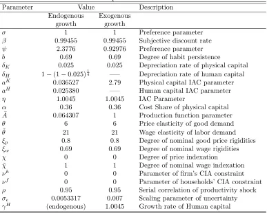
The parameter values are summarized in Table 1. The deep parameters are calibrated by the following way. The time unit is assumed to be one quarter. We assume cashless economy so that νh and νf is zero. σ is set to be 1, that
is, we assume that log utility. Given that, we divide the parameters to be calibrated into three groups. For parameters in the first group, b, δK, δH, α,
θ, ˜θ, ξp, ξw, χ, ˜χ, and ρ, we draw on related studies. ρ are set to be 0.95,
which are in the range of the value used in RBC literature. We set b to be 0.69, δK to be 0.025,α to be 0.36, ˜θto be 21,ξp to be 0.8, and ξw to be 0.69,
following Altig et al. (2005). δH is assumed to be 1−(1−0.025)1/4, following
Jones et al. (2005a). θ is assumed to be 6, such that the steady-state markup in product good markets is 20 percent. Following SGU and the empirical fact found by Levin et al. (2005), we set χ and ˜χ to be 0 and 1, respectively.
Second, given the values set above, parameters in the second group, which is composed ofψ,η, ¯A, are calibrated by using steady-state conditions and some restrictions. We think zero-inflation steady-state and assume that steady-state output growth rate is 0.45 percent per quarter, following SGU. In the deterministic steady state, we assume labor supply,n, to be one half,6
5See Jones and Manuelli (1990), for more general formulation.
Table 1: Deep Structural Parameters
Parameter Value Description
Endogenous Exogenous growth growth
σ 1 1 Preference parameter
β 0.99455 0.99455 Subjective discount rate
ψ 2.3776 0.92976 Preference parameter
b 0.69 0.69 Degree of habit persistence
δK 0.025 0.025 Depreciation rate of physical capital
δH 1−(1−0.025)
1
4 —– Depreciation rate of human capital
aK 0.036527 2.79 Physical capital IAC parameter
aH 0.025380 —– Human capital IAC parameter
η 1.0045 1.0045 IAC Parameter
α 0.36 0.36 Cost Share of physical capital ¯
A 0.064307 1 Production function parameter
θ 6 6 Price elasticity of good demand ˜
θ 21 21 Wage elasticity of labor demand
ξp 0.8 0.8 Degree of nominal good price rigidities
ξw 0.69 0.69 Degree of nominal wage rigidities
χ 0 0 Degree of price indexation
˜
χ 1 1 Degree of nominal wage indexation
νh 0 0 Parameter of firm’s CIA constraint
νf 0 0 Parameter of households’ CIA constraint
ρ 0.95 0.95 Serial correlation of productivity shock
σǫ 0.0053317 0.007 Scaling parameter of uncertainty
γH (endogenous) 1.0045 Growth rate of Human capital
quarterly real interest rate, rK, to be one percent, each price of physical and
human capital, qK and qH, to be 1, respectively. Under these assumptions,
we obtain the values of ψ, η, and ¯A by using steady-state conditions. Finally, parameters in the third group,aK,aH, andσ
ǫ, are calibrated such
that the second moment of key variables in the model match the U.S. business cycle fact. We set these values such that standard deviation of output growth rate is 0.84, that standard deviation of physical capital investment growth is three times larger than that of output growth, and that standard deviation of broad consumption7 growth is as half as that of output growth under simple
Taylor rule with zero inflation target, log(Rt/R¯) = 1.5 logπt.
For comparative purpose, we also consider the counterpart exogenous growth model. In the exogenous growth model, the growth rate of human capital, γH
t , is exogenously 1.0045 in all t and human capital investment is
zero. aH no longer affects the equilibrium. aK is set to be 2.79, following
7Following Jones et al. (2005a), we refer the sum of consumption and human capital
SGU. σǫ is set to be 0.007, which is standard RBC literature. Given that,
We calibrate the parameters of the exogenous growth model by the same steady-state restrictions as the endogeous growth model.8
3
Steady State Analysis
3.1
Optimal Long-run Inflation Rate
Given our assumptions of cashless economy, tax on human capital investment, subsidies on employment and production, no price indexation, and full wage indexation, we ensure that real allocation of the deterministic steady state at zero inflation is the same as steady-state real allocation of social planner solution. Therefore, the deterministic steady state at zero inflation is Pareto optimal.
3.2
Growth and Welfare effect of Long-run Inflation
Despite some empirical studies claim the importance of the negative corre-lation between long-run growth and infcorre-lation, it is underestimated in theo-ritical literature using nominal frictions such as cash-in-advance constraints. For example, Kormendi and Meguire (1985) estimated their correlations us-ing cross-country data and found that a decreasus-ing of inflation by 2% would rise the growth rate by 1% per annum, but in theorictical analysis, com-puted growth effect caused by 10% increasing of annual inflation rate lowers the annual growth rate by only 0.06% in Gomme (1993) and 0.3% in Jones and Manuelli (1995). In contrast, the sticky price model has the more sig-nificantly negative growth and welfare effect of inflation than their flexible price models. Figure 1 represents the relationship between growth and in-flation in the deterministic steady steady state. In our baseline calibration, a increasing of inflation from 0% to 10% lowers growth by about 1% per annum. Moreover, we find that in our model, welfare cost of inflation is also large. a increasing of inflation by 10% per annum decreases economic welfare by more than 30% consumption measured at zero-inflation (Pareto-optimal) steady state.
Our result obtained above shows that price stickiness brings the signif-icant growth and welfare effect.9 The degree of price stickiness, however,
8The scaling parameter of production function, ¯A, is arbitary in the exogenous model.
Without loss of generality, we set ¯A= 1.
9Wage stickiness does not cause growth and welfare effects in steady state of our model
Fig. 1: The effects of long-run inflation
−4 −2 0 2 4 6 8 10 0
10 20 30
40 Welfare Cost
−4 −2 0 2 4 6 8 10 0.85
0.9 0.95 1 1.05
Real Marginal Cost
−4 −2 0 2 4 6 8 10 2.5
3 3.5 4
4.5 Real Interest Rate
−4 −2 0 2 4 6 8 10 0.5
1 1.5
2 Real Growth Rate
−4 −2 0 2 4 6 8 10 6.4
6.5 6.6 6.7 6.8 6.9 7
x 10−3Consumption
−4 −2 0 2 4 6 8 10 0.475
0.48 0.485 0.49 0.495 0.5 0.505
Table 2: The growth and welfare effect of 10% annual inflation ξp 0.2 0.4 0.6 0.8 (baseline)
Growth effect -0.007 -0.0257 -0.102 -1.03 Welfare cost 0.255 0.983 3.92 35.5
Note: i) Growth rate is described in net growth per year. ii) Welfare cost is measured by percentage of consumption in zero-inflation steady state.
would be highly difference across countries. We then do a sensitivity analy-sis for the degree of price stickiness,ξp. Table 2 represents growth and welfare
effect of 10% annual inflation when ξp = 0.2,0.4,0.6,0.8. The result shows
that the low degree of price stickiness lower the growth effect of inflation. Note that growth and welfare effect is nonlinear in our model. The higher inflation is, the more marginal growth decreasing is. This nonlinearity is not consistent with recent empirical evidence. We conjecture that our nonlinear-ity result is caused by the time-dependent sticky price assumption. In the assumption, high inflation bring severe distortion of price stickiness. If the assumption of sticky price was state-dependent pricing such as Dotsey et al. (1999), high inflation would lower the degree of price stickiness and might be consistent with empirical studies.
4
Equilibrium Dynamics
4.1
Solution Method
Because of the complexity of the model, an exact numerical solution does not exist. The log-linearization method, however, eliminates the growth effects which comes from uncertainty because unconditional means of en-dogenous variables are identical to the values at deterministic steady state in log-linearized model. We then approximate the equilibrium conditions and the conditional welfare measure to second-order accuracy by using the computation method developed by Schmitt-Grohe and Uribe (2004).
4.2
Monetary Policy Rules
We consider the equilibrium dynamics and welfares under simple Taylor rule and optimal operational monetary policy rules below. In this subsection, we present the definitions of Taylor rules.
The Simple Taylor Rule First, as a benchmark, we apply the simple Taylor rule responding only to inflation,
log
(
Rt
R∗
)
= 1.5 log(πt π∗
)
, (49)
where variables with asterisks denote their values at the zero-inflation deter-ministic steady state.
The Taylor Rule In order to investigate the effect of growth by respond-ing to output, we use the standard Taylor rule also respondrespond-ing to cyclical components of output,
log
(
Rt
R∗
)
= 1.5 log(πt π∗
)
+ 0.5 log
(
yt
y∗
)
. (50)
4.3
Results
4.3.1 Growth effects of Monetary Policy
Our numerical result under the simple and standard Taylor rules are repre-sented in Table 3. According to this, under baseline parameters the simple Taylor rule lowers the long-run growth rate by 3×10⁻³
percent per year. Furthermore, the rule responding to output has more significantly negative growth effect. the rule lowers the long-run growth rate by 7×10⁻²
percent per year. It is seen to be small for policy implication but we think it as not to be negligible for the literature of the relationship between growth and fluctuations. For example, Jones et al. (2005b) show that the convex mod-els of endogenous growth without nominal rigidities has positive or negative growth effect of uncertainty. Under reasonable parameter values, the growth effects of uncertainty in their model increase long-run growth rate by at most 7×10⁻²
percent per year. Hence, the growth effects of monetary policy at least offset their growth effect when the economies have nominal rigidities. Jones et al. (2005b) claim that the differences of long-run growth across countries may be able to contribute to sharper estimations of deep param-eters such as intertemporal elasticity of substitution. Our result, however, suggests that given the existence of nominal rigidities and the differences of policy rules across countries, we can not ignore the growth effect of the differences of monetary policy rules to estimate those ones.
4.3.2 Relationship between Inflation Volatility and Growth
Fig. 2: The inflation volatility effects on long-run growth
0 1 2 3
0 1 2 3
απ
α
π
W
o
b
o:welfare,+:E(γY
),x:σ(π), Welfare
απ
α
π
W
o
b
0 1 2 3
0 1 2 3
E(γY
)
απ
α
π
W
o
b
0 1 2 3
0 1 2 3
σ(π)
απ
α
π
W
o
b
0 1 2 3
0 1 2 3
σ(πWo b
)
απ
α
π
W
o
b
0 1 2 3
0 1 2 3
σ(R)
απ
α
π
W
o
b
0 1 2 3
Table 3: The Taylor Rules
Simple Taylor Rule: log(Rt/R∗) = 1.5 log(πt/π∗)
Taylor Rule - Output: log(Rt/R∗) = 1.5 log(πt/π∗) + 0.5 log(yt/y∗)
Welfare Cost σπ σπW ob σR E(ˆγY)
A: Endogenous Growth New Keynesian Model Baseline
Simple Taylor Rule 0.073 0.38 1.12 0.57 −2.61×10⁻³
Taylor Rule - Output 4.005 5.56 5.52 5.32 −7.74×10⁻²
High IACs (aK=aH= 10)
Simple Taylor Rule 0.058 0.86 0.58 1.29 −2.81×10⁻³
Taylor Rule - Output 4.300 5.77 5.77 6.12 −8.41×10⁻²
B: Standard New Keynesian Model Baseline
Simple Taylor Rule 0.011 0.79 0.64 1.19 — Taylor Rule - Output 3.189 7.99 8.01 8.30 — High IAC (aK= 10)
Simple Taylor Rule 0.029 1.09 0.73 1.63 — Taylor Rule - Output 3.042 7.83 7.87 8.29 —
Note: i) For definition of welfare cost, see appendix. ii)σxrepresents the standard
deviation ofx. σπ,σR denote on annual rates. iii)E(ˆc) represents unconditional mean of
percentage deviation ofc from deterministic steady state. E(ˆγY) denotes unconditional
mean of percentage deviation ofγY from deterministic steady state on annual rate.
however, implies unclear correlations across countries. In our model, their relationship depends on the monetary policy rules. We here consider the following rule,
log
(
Rt
R∗
)
=απlog(πt π∗
)
+απW ob log
(
πWob
t
πWob∗ )
, (51)
where we define the observable nominal wage inflation,πWob
t , as
πWt ob ≡ WtHt
Wt−1Ht−1
=πtγtH
wt
wt−1
.
Figure 2 shows that the relationship between policy coefficients which govern response to price- and wage-inflation and the moments of relavant endogenous variables. When απW ob
is high, long-run growth has negative relationship to inflation volatility. However, When απW ob
is relatively low, the two has positive relationship because then the higher απ is, the smaller
σ(π) is but the greater volatility of wage inflation σ(πWob
[image:22.595.108.431.504.598.2]Table 4: Optimal Operational Monetary Policy Rules Policy Coefficients σπ σπW ob σR E(ˆγY)
απ αγY
απWob
αR
A: Endogenous Growth New Keynesian Model
Baseline 1.70 0.00 0.89 0.00 0.28 0.42 0.27 1.7×10⁻⁴
High IACs
aK=aH = 10 6.52 0.00 6.28 0.00 0.41 0.34 1.30 −1.1×10⁻³
B: Standard New Keynesian Model
Baseline 2.70 0.00 0.15 0.04 0.52 0.57 1.39 — High IACs
aK= 10 3.68 0.00 2.31 0.00 0.59 0.52 1.41 —
Note: i) For definition of policy rule, see equation (52). ii)σx represents the standard
deviation ofx. σπ,σR denote on annual rates. iii)E(ˆc) represents unconditional mean of
percentage deviation ofc from deterministic steady state. E(ˆγY) denotes unconditional
mean of percentage deviation ofγY from deterministic steady state on annual rate.
5
Optimal Operational Monetary Policy Rules
5.1
Definition
The operational monetary policy rules are defined as the rules satisfying the following four operational conditions similar to SGU. First, monetary orthority must set nominal interest rate according to the following interest rate feedback rules,
log
(
Rt
R∗
)
=απlog(πt
π∗
)
+αγY log
(
γY t
γY∗
)
+απW ob log
(
πWob
t
πWob∗ )
+αRlog
(
Rt−1
R∗
)
,
(52) Second, coefficients of the interest rate rules, απ, αγY
, απW ob
, and αR,
must be in the ranges of [0,10]. Third, The equilibrium must be uniquely determined, that is, equilibrium under operational policy must not have fluc-tuation driven by agents’ expectations. Fourth, The standard deviation of nominal rate of interest must be less than a half of steady state value of nominal interest rate, that is, 2σR < logR∗, that is, the possibilities that
nominal interest rate hits its zero-lower bound must be kept to be low. In this section, we consider optimal operational monetary policy rules of our model. Assume that the economy is in the deterministic steady state at the beginning of period 0. The optimal policy (απ αγY
απW ob
αR) maximizes
as
vt=
β
1−β logγ
H
t+1+ log(ct−bct−1/γ
H
t ) +ψlog(1−nt) +βEtvt+1, (53)
subject to the operational conditions defined above. This conditional wel-fare measure is derived from the utility function of representative household. The details are in appendix. We analyze the optimal policy under baseline structural parameter values.
Moreover, we compute the optimal policy under the high investment ad-justment cost case, aK = aH = 10. The reasons is as follows. First, we
calibrate the parameters which govern the degrees of investment adjustment cost to match the ratio of volatility of physical capital investment and the ratio of volatility of broad consumption to the volatility of output. However, we have not empirical evidence enough to estimate the degrees of investment adjustment cost sharply, especially human capital investment adjustment cost. Hence, we would have to do sensitivity analysis about their parame-ter. Second, more importantly, investment adjustment costs theirselves have the growth effect of investment volatility. Barlevy (2004b) shows that in the endogenous growth models with concave capital production technolo-gies, equivalently convex investment adjustment costs, investment volatili-ties lower long-run growth even if unconditional means of investment levels unchange. Therefore, if the model has a negative relationship between price-or wage-stabilization and investment stabilization, Optimal policy rules may respond to output when Barlevy’s effect is strong. The socond reason is that we would like to investigate whether optimal monetary policy is changed by Barlevy’s effect.
5.2
Results
Our numerical results are shown in Table 4. Under the baseline calibration, the response of optimal monetary policy rules to price and wage inflation are positive, and the one to output growth is mute. This result is simi-lar to the exogenous growth model with sticky price and wage. SGU and Schmitt-Grohe and Uribe (2007) show that optimal operational monetary policy should respond to inflation and should not respond to output or out-put growth. The reason is that the larger policy coeffcient with respect to output growth,αγY
, is, the greater volatility of inflation is so that the distor-tion of price dispersion becomes higher. We see the fact that this intuidistor-tion is right by the analogy to Table 3.
Our second finding is that optimal monetary policy virtually does not
Table 5: Growth-Maximizing Monetary Policy Rules
Policy Coefficients Welfare σπ σπW ob σR E(ˆγY)
απ αγY
απWob
αR Cost
(100×Λc)
Baseline 1.37 0.00 0.83 0.00 4.4×10⁻⁴ 0.25 0.46 0.26 1.9×10⁻⁴
High IACs
aK =aH= 10 5.27 0.00 4.88 0.00 8.4×10⁻⁵ 0.43 0.33 1.27 −1.1×10⁻³
Note: i) For definition of policy rule, see equation (52). ii)σx represents the standard
deviation ofx. σπ,σR denote on annual rates. iii)E(ˆc) represents unconditional mean of
percentage deviation ofc from deterministic steady state. E(ˆγY) denotes unconditional
mean of percentage deviation ofγY from deterministic steady state on annual rate.
adjustment costs are extremely high, aK =aH = 10, the features of optimal
policy regime that monetary authority should respond to price- and wage-inflation and not to real activity does not change.
These two findings suggest that growth effect itself have only weak trade-off between price- and wage- inflation stabilization descrived in the previ-ous subsection because optimal policy rules feature only price- and wage-stabilization. In order to ensure that growth effect of investment adjustment costs, we do an exercise seeking operational monetary policy rules maximize the unconditional mean of output growth. The result represents in Table. 5. We find that the growth-maximizing policy rule responds only to price-and wage-inflation price-and not to output growth price-and this rule atteins virtually identical long-run output growth rate to that of optimal policy rule. This re-sult suggests that our conclusion that Barlevy’s effect has not strong tradeoff between nominal and investment stabilization would be right.
6
Conclusion
This paper analyses the effects of monetary policy in an endogenous growth model. In this paper, we obtain some positive and normative implications about inflation and growth. First, in steady state, sticky price distortion have the negative growth and welfare effect and this effect is highly sensitive to the degree of price stickiness. This sensitivity may account for the difference of growth rate across countries. Of cource, price stickiness would change along the economic environment and time so that we need further theoretical and empirical studies about price stickiness.
affected by the monetary stabilization policy rules. Especially, policy rule responds to output lower the long-run growth rate strongly. The empirical study by Orphanides (2003) suggests the possiblities that output response of monetary policy in the Great Inflation period brings stagflation. Our numerical result is consistent with his findings. The simulation analysis using our model about the periods would be useful to understand the mechanism of stagflation.
Third, The effect of volatility of inflation on long-run growth is not clear. This result is consistent with empirical evidence. The source of unclearness in our model is the existence of wage stickiness. Our conclusion should be tested by an empirical exercise about the relationship between inflation volatility and growth, in addition to wage volatility.
Fourth, in spite of above various results that growth and nominal vari-ables, the features of the optimal operational policy is not turned from exoge-nous growth New Keynesian models. Our numerical exercises demonstrate that resolution of price- and wage- tradeoff virtually maximize the long-run growth. This result implies that the tradeoff between stabilization and growth does not exist or is weak. This conclusion is also very similar to Black-burn and Pelloni (2005). They show that in an endogenous growth model with sticky wage, growth-maximizing policy is optimal. Our result implies that growth is important from positive perspective but monetary authorities do not need to consider growth in practice.
Appendix A: Equilibrium Conditions
Equilibrium conditions
Λt[1 +νh(1−R−t1)] = (Ct−bCt−1)−σ(1−nt)ψ(1−σ)−βbEt(Ct+1−bCt)−σ(1−nt+1)ψ(1−σ)
1
Rt
=βEt
Λt+1
Λtπt+1 Yt=Ct+ItK+ItH
θX1
t = (θ−1)Xt2
Xt1= ˜p−θ−1
t Ytmct+ξpβEt
Λt+1
Λt
( πχ
t
πt+1
)−θ( p˜
t
˜
pt+1
)−θ−1
Xt1+1
Xt2= ˜p−tθYt+ξpβEt
Λt+1
Λt
(
πtχ
πt+1
)1−θ(
˜
pt
˜
pt+1
)−θ
Xt2+1
1 = (1−ξp)˜p1t−θ+ξp
(πχ
t−1 πt
)1−θ
AtKtα(ndt)1−αHt1−α=Ytst
st= (1−ξp)˜p−tθ+ξp
(πχ
t−1 πt
)−θ
st−1
rK
t =αAtKtα−1(ndt)
1−αH1−α t mct
wt[1 +νf(1−R−t1)] = (1−α)AtKtα(ndt)−αHt−αmct
Ft1=
˜
θ−1 ˜
θ Λtn
d tHt
(w˜
t
wt
)−θ˜
˜
wt+βξwEt
( w˜
t
˜
wt+1
)1−θ˜( πχ˜
t
πt+1
)1−θ˜
Ft1+1
F2
t =ndt
(w˜
t
wt
)−θ˜
ψ(Ct−bCt−1)1−σ(1−nt)ψ(1−σ)−1+βξwEt
( w˜
t
˜
wt+1
)−θ˜( πχ˜
t
πt+1
)−θ˜
F2
t+1 Ft1=Ft2
nt=ndts˜t
˜
st= (1−ξw)
(w˜
t
wt
)−θ˜
+ξw
(w
t−1 wt
)−θ˜(πχ˜
t−1 πt
)−θ˜
˜
st−1
w1−θ˜
t = (1−ξw) ˜w1−
˜
θ t +ξw
(
πtχ˜−1 πt
)1−θ˜
w1−θ˜ t−1 Mt=νhCt+νfwtndtHt
Kt+1= (1−δK)Kt+ItK−
aF K
2
( IK t
IK t−1
−ηF K
)2
IK t
Ht+1= (1−δH)Ht+ItH−
aF H
2
( IH t
IH t−1
−ηF H
)2
IH t
Λt= ΛtqtK
[
1−a
F K
2
(IK t
IK t−1
−ηF K
)2
−aF K
(IK t
IK t−1
−ηF K
) IK t
IK t−1
]
+βEtΛt+1qKt+1aFK
(IK t+1 IK
t
−ηF K
) (IK t+1 IK
t
Λt= ΛtqtH
[
1−a
F H
2
( IH t
IH t−1
−ηF H
)2
−aF H
( IH t
IH t−1
−ηF H
) IH t
IH t−1
]
+βEtΛt+1qHt+1aFH
(IH t+1 IH
t
−ηF H
) (IH t+1 IH
t
)2
ΛtqKt =βEtΛt+1[rKt+1+qtK+1(1−δK)]
ΛtqHt =βEtΛt+1[wt+1ndt+1+qtH+1(1−δH)]
Equilibrium conditions written by stationary variables
γH
t+1kt+1= (1−δK)kt+iKt −
aF K
2
(γH t iKt
iK t−1
−ηF K
)2
iK t
γH
t+1= 1−δH+iHt −
aF H
2
(
γH t iHt
iH t−1
−ηF H
)2
iH t
λt=λtqKt
[
1−a
F K
2
(
γH t iKt
iK t−1
−ηF K
)2
−aF K
(
γH t iKt
iK t−1
−ηF K
)
γH t iKt
iK t−1
]
+βEt(γHt+1)−σλt+1qKt+1aFK
(γH t+1iKt+1
iK t
−ηF K
) (γH t+1iKt+1
iK t
)2
λt=λtqHt
[
1−a
F H
2
(γH t iHt
iH t−1
−ηF H
)2
−aF H
(γH t iHt
iH t−1
−ηF H
)γH t iHt
iH t−1
]
+βEt(γHt+1)−σλt+1qHt+1aFH
(γH t+1iHt+1
iH t
−ηF H
) (γH t+1iHt+1
iH t
)2
λt[1 +νh(1−R−t1)] = (ct−bct−1/γtH)−σ(1−nt)ψ(1−σ)−βbEt(γtH+1ct+1−bct)−σ(1−nt+1)ψ(1−σ) λtqtK=βEt(γtH+1)−σλt+1[rKt+1+qKt+1(1−δK)]
λtqtH=βEt(γtH+1)−σλt+1[wt+1ndt+1+qtH+1(1−δH)]
1
Rt
=βEt
(γH
t+1)−σλt+1 λtπt+1 yt=ct+iKt +iHt
θx1t = (θ−1)x2t
x1t = ˜pt−θ−1ytmct+ξpβEt
λt+1 λt
(γH t+1)1−σ
(
πχt
πt+1
)−θ(
˜
pt
˜
pt+1
)−θ−1
x1t+1
x2
t = ˜p−tθyt+ξpβEt
λt+1 λt
(γH t+1)1−σ
( πχ
t
πt+1
)1−θ( p˜
t
˜
pt+1
)−θ
x2
t+1
1 = (1−ξp)˜p1t−θ+ξp
(πχ
t−1 πt
)1−θ
Atkαt(ndt)1−α=ytst
st= (1−ξp)˜p−tθ+ξp
(πχ
t−1 πt
)−θ
st−1
rK
t =αAtkαt−1(ndt)1−αmct
ft1= θ˜−1 ˜
θ λtn
d t
(w˜
t
wt
)−θ˜
˜
wt+βξwEt
( w˜
t
˜
wt+1
)1−θ˜( πχ˜
t
πt+1
)1−θ˜
(γH
t+1)1−σft1+1
ft2=nd t
(w˜
t
wt
)−θ˜
ψ(ct−bct−1/γtH)
1−σ(1−n
t)ψ(1−σ)−1+βξwEt
( w˜
t
˜
wt+1
)−θ˜( πχ˜
t
πt+1
)−θ˜
(γH
t+1)1−σft2+1 ft1=ft2
nt=ndts˜t
˜
st= (1−ξw)
(w˜
t
wt
)−θ˜
+ξw
(w
t−1 wt
)−θ˜(πχ˜
t−1 πt
)−θ˜
˜
st−1
w1t−θ˜= (1−ξw) ˜w1−
˜
θ t +ξw
(
πtχ˜−1 πt
)1−θ˜
w1t−−1θ˜
mt=νhct+νfwtndt
log (R t ¯ R )
=απlog
(πt
¯
π
)
+αγY log
(γY t
¯
γY
)
+αRlog
(R
t−1
¯
R
)
γY t =γtH
yt
yt−1
Deterministic steady state
(γH−1 +δK)k=iK
[
1−a
F K
2 (γ
H−ηF K)2
]
γH = 1−δH+iH
[
1−a
F H
2 (γ
H−ηF H)2
]
1 =qK
[
1−a
F K
2 (γ
H−ηF
K)2−aFK(γH−ηKF)γH
]
+β(γH)2−σqKaF
K(γH−ηKF)
1 =qH
[
1−a
F H
2 (γ
H−ηF
H)2−aFH(γH−ηFH)γH
]
+β(γH)2−σqHaF
H(γH−ηHF)
λ[1 +νh(1−R−1)] =c−σ(1−n)ψ(1−σ)(γH−b)−σ[(γH)σ−βb]
qK=β(γH)−σ[rK+qK(1−δ K)]
qH=β(γH)−σ[wnd+qH(1−δ H)]
R= (γ
H)σπ
β y=c+iK+iH
x1= ˜p−θ−1ymc+ξ
pβ(γH)1−σπ−θ(χ−1)x1
x2= ˜p−θy+ξ
pβ(γH)1−σπ(1−θ)(χ−1)x2
θx1= (θ−1)x2
1 = (1−ξp)˜p1−θ+ξpπ(1−θ)(χ−1)
¯
s= (1−ξp)˜p−θ+ξpπ−θ(χ−1)s
rK= αysmc
k
w[1 +νf(1−R−1)] =(1−α)ysmc nd
f1= θ˜−1
˜
θ λn
d
(w˜
w
)−θ˜
˜
w+βξwπ(˜θ−1)(1−χ˜)(γH)1−σf1
f2=nd
(w˜
w
)−˜θ
ψc1−σ(γH)σ−1(γH−b)1−σ(1−n)ψ(1−σ)−1+βξ
wπ
˜
θ(1−χ˜)(γH)1−σf2
f1=f2
n=nds˜
˜
s= (1−ξw)
(w˜
w
)−˜θ
+ξwπ
˜
θ(1−χ˜)˜s
w1−θ˜= (1−ξ w) ˜w1−
˜
θ+ξ
wπ(˜θ−1)(1−χ˜)w1−
˜
θ
γY =γH
m=νhc+νfwnd
Appendix B: Welfare Cost Measure
CRRA case
Vt ≡Et
∞
∑
s=0
βs(Ct+s−bCt+s−1)
1−σ
(1−nt+s)ψ(1−σ)
1−σ
= (Ct−bCt−1)
1−σ
(1−nt)ψ(1−σ)
1−σ +βEtVt+1
Dividing it by H1−σ
t and defining vt= HV1t−σ
t , we rewrite the welfare function as the recursive formulation by the stationary variables:
vt =
(ct−bct−1/γtH)1 −σ
(1−nt)ψ(1−σ)
1−σ +β(γ
H t+1)1
−σ
Etvt+1.
log case (σ = 1)
Vt≡Et
∞
∑
s=0
βs[log(Ct+s−bCt+s−1) +ψlog(1−nt+s)]
= 1
1−β logHt+Et
∞
∑
s=0
[
β
1−β logγ
H
t+1+s+ log(ct+s−bct+s−1/γ
H
t+s) +ψlog(1−nt+s)
Defining vt as:
vt ≡Vt−
1
1−βlogHt, we obtain the recursive formulation:
vt =
β
1−β logγ
H
t+1+ log(ct−bct−1/γ
H
t ) +ψlog(1−nt) +βEtvt+1.
Reference
Altig, David, Lawrence J. Christiano, Martin Eichenbaum, and Jesper Linde (2005) “Firm-Specific Capital, Nominal Rigidities, and the Business Cy-cle.” NBER Working Paper No. 11034.
Barlevy, Gadi (2004a) “The Cost of Business Cycles and The Benefit of Stabilization: A Survey.” NBER Working Paper, No. 10926.
Barlevy, Gadi (2004b) “The Cost of Business Cycles Under Endogenous Growth,” American Economic Review, Vol. 94, No. 4, pp. 964–990.
Blackburn, Keith and Alessandra Pelloni (2005) “Growth, Cycles, and Sta-bilization Policy,” Oxford Economic Papers, Vol. 57, pp. 262–282.
Calvo, Guillermo (1983) “Staggered Prices in a Utility-Maximizing Frame-work,”Journal of Monetary Economics, Vol. 12, No. 3, pp. 383–398.
Christiano, Lawrence J., Martin Eichenbaum, and Charles L. Evans (2005) “Nominal Ligidities and the Dynamic Effects of a Shock to Monetary Pol-icy,” Journal of Political Economy, Vol. 113, pp. 1–45.
Comin, Diego and Mark Gertler (2006) “Medium-Term Business Cycles,”
American Economic Review, Vol. 96, No. 3, pp. 523–51.
Dotsey, Michael and Pierre D. Sarte (2000) “Inflation Uncertainty and Growth in a Cash-in-advance Economy,” Journal of Monetary Economics, Vol. 45, pp. 631–655.
Gomme, Paul (1993) “Money and Growth Revisited: Measuring the Cost of Inflation in an Endogenous Growth Model,” Journal of Monetary Eco-nomics, Vol. 32, pp. 51–77.
Jones, Larry E. and Rodolfo E. Manuelli (1990) “A Convex Model of Equi-librium Growth: Theory and Policy Implications,” Journal of Political Economy, Vol. 98, No. 1, pp. 1008–1038.
Jones, Larry E. and Rodolfo E. Manuelli (1995) “Growth and the Effects of Inflation,” Journal of Economic Dynamics and Control, Vol. 19, pp. 1405–1428.
Jones, Larry E., Rodolfo E. Manuelli, and Henry E. Siu (2005a) “Fluctuations in Convex Models of Endogenous Growth, II: Business Cycle Properties,”
Review of Economic Dynamics, Vol. 8, pp. 805–828.
Jones, Larry E., Rodolfo E. Manuelli, Henry E. Siu, and Ennio Stacchetti (2005b) “Fluctuations in Convex Models of Endogenous Growth, I: Growth Effects,” Review of Economic Dynamics, Vol. 8, pp. 780–804.
Kormendi, Roger C. and Phillip G. Meguire (1985) “Macroeconomic Deter-minants of Growth: Cross-country Evidence,” Journal of Monetary Eco-nomics, No. 16, pp. 141–163.
Levin, Andrew T., Alexei Onatski, John C. Williams, and Noah Williams (2005) “Monetary Policy Under Uncertainty in Micro-Founded Macroe-conometric Models.” manuscript prepared for the NBER’s Twentieth An-nual Conference on Macroeconomics.
Lucas, Robert E. (1987)Models of Business Cycles, Oxford: Basil Blackwell.
Lucas, Robert E. (2003) “Macroeconomic Priorities,” American Economic Review, Vol. 93, No. 1, pp. 1–14.
Orphanides, Athanasios (2003) “Historical Monetary Policy Analysis and the Taylor Rule,” Journal of Monetary Economics, Vol. 50, No. 3, pp. 983– 1022.
Schmitt-Grohe, Stephanie and Martin Uribe (2005) “Optimal Inflation Stabi-lization in a Medium-Scale Macroeconomic Model.” NBER Working Paper, No. 11854.
Schmitt-Grohe, Stephanie and Martin Uribe (2007) “Optimal Simple and Im-plementable Monetary and Fiscal rules,”Journal of Monetary Economics, Vol. 54, pp. 1702–1725.