Measuring the Dynamic Cost of Living Index from Consumption Data

Munich Personal RePEc Archive

Measuring the Dynamic Cost of Living

Index from Consumption Data

Aoki, Shuhei and Kitahara, Minoru

Graduate School of Economics, University of Tokyo, Population

Research Institute, Nihon University

2 August 2008

Online at

https://mpra.ub.uni-muenchen.de/9802/

Measuring the Dynamic Cost of Living Index

from Consumption Data

∗

Shuhei Aoki

Minoru Kitahara

August 2, 2008

Abstract

In the U.S., the objective of consumer price index (CPI)

measure-ment is to measure the cost of living. However, the current CPI or, in

other words, cost of living index (COLI) measures the cost of living

in a static optimization problem. This paper proposes a new method

to construct a dynamic cost of living index (DCOLI). Our method

offers several advantages compared to other dynamic cost of living

in-dices proposed in the literature. First, our measure is based on total

wealth. Previous indices limited attention to financial wealth.

Sec-ond, we consider an Epstein-Zin preference structure. Most previous

∗_{We are indebted to Toni Braun for his help in the inital stages of this research. All}

remaining errors are, of course, our own.

†_{Graduate School of Economics, University of Tokyo, 7-3-1, Hongo, Bunkyo-ku, Tokyo}

113-0033, Japan. Email: shuhei [email protected]

‡_{Population Research Institute, Nihon University, 12-5, Goban-cho, Chiyoda-ku, Tokyo}

literature has used log preferences. We derive formulas that relate

our DCOLI to the COLI and derive conditions under which the two

coincide. We also produce empirical measures of our DCOLI. We find

that under standard assumptions on preferences, the volatility of our

DCOLI is about the same as that of the COLI. In certain periods,

e.g., 1977–1983, our measure differs sharply from the COLI.

JEL classification: E31, C43, D91.

Keywords: dynamic cost of living index; cost of life; CPI.

1

Introduction

The Consumer Price Index (CPI) is the most widely used measure of the general price level in the U.S. Taxes, welfare payments, retirement payments, and labor contracts are all indexed to the CPI. Stabilizing CPI growth is a central objective of monetary policy.

In the U.S., it is generally accepted that the objective of CPI measurement is to measure changes in the purchasing power of money (for details, see, e.g., the Bureau of Labor Statistics (2007)). That is, the CPI is a “cost of living” index (COLI). Changes in a cost of living index are defined as the ratio of the expenditure function evaluated at different prices. Current COLI measurement implicitly assumes that the expenditure function is associated with a static expenditure minimization problem.

should reflect not just the price of today’s goods but also that of future goods. Alchian and Klein (1973) point out this problem and propose a dynamic cost of life index (DCOLI) that recognizes that the money cost of goods includes the cost of future goods as well as that of current goods. Pollak (1975) provides a general theoretical treatment of intertemporal price indices.

A DCOLI has some very attractive properties. A DCOLI measures the money cost of yielding a reference level of lifetime utility. If a change in prices leads to an increase in the DCOLI, it implies that the money cost of goods has risen. In other words, the lifetime utility delivered by the reference level of nominal wealth has fallen. In situations where households are active for many periods, the properties of a DCOLI can, in principle, differ substantially from those of a COLI, which just focuses on current period utility.

However, there are some major obstacles to measuring a DCOLI. One ob-stacle emphasized by Alchian and Klein (1973) is measuring nominal wealth. In principle, one needs futures prices for each component of nominal wealth. Due to the absence of markets for these goods, one has to infer their prices indirectly by imposing restrictions on preferences and assuming complete markets.

price shock in 1973 and also between 1985 and 1990. Shiratsuka (1999) relaxes the assumption of constant real returns and addresses the question of whether a DCOLI should be used when setting monetary policy. His answer to this question is negative: he suggests that a DCOLI is considerably more volatile than the GDP deflator; that the reliability of the measurement of certain assets used to construct the DCOLI in the previous literature, such as land and house prices that receive large weight in wealth, is low; and that asset prices may respond to variations in spurious variables (e.g., sunspots). Reis (2005) constructs a DCOLI using U.S. data and also finds that it is much more volatile than the COLI. These problems have led Bryan et al. (2001) to adopt an empirical approach for measuring the dynamic cost of life that combines some restrictions from theory with an econometric approach for identifying good indicators of future prices. One feature common to all this previous research is that human wealth is not used when constructing the measure of the DCOLI. Shiratsuka (1999) points out that the human wealth component is large but argues that it is hard to measure and only reports results for a DCOLI that uses financial wealth.

the sense that they do not have to take an explicit position on the expected returns on human wealth or its growth rate. They find that the volatility of human wealth and thus total wealth is considerably lower than that of financial wealth. A common theme underlying this entire literature is that restrictions from preferences are not used to restrict the dynamics of human wealth.

One contribution of this paper is that we use restrictions from preferences to identify and estimate both human and total wealth. We adopt a specific preference structure, assume complete markets, and derive a stochastic pric-ing kernel. Then, we use this pricpric-ing kernel to value dividends on human and financial wealth.

We also consider a class of preferences that is more general than that used in the previous literature on DCOLI measurement. Shibuya (1992) and Shiratsuka (1999) both assume log preferences. Reis (2005) uses log preferences for most of his analysis but considers a generalization to Epstein-Zin preferences. His analysis of this case imposes the assumption that equity prices follow a random walk and that goods prices follow an AR(1) in first differences. In addition, he does not produce an empirical measure for this preference structure.

static problem and the real dynamic cost of living index (RDCOLI). We find that when the EIS (elasticity of intertemporal substitution) is very large, the DCOLI coincides with the COLI. Our DCOLI also has the property that its long-run growth rate coincides with that of the COLI.

We now summarize our empirical results. First, there are sharp differences between the COLI and DCOLI in 1973–1976 and 1977–1983, i.e., around the time of the first and second oil crises. During these periods, the RDCOLI, which is equal to the DCOLI minus the COLI, experienced the sharpest decline. This indicates that the prices of future goods sharply fell or, in other words, the expected future returns on total wealth increased. Second, contrary to the previous research, the volatility of our DCOLI is about the same as that of the COLI. We find that the difference between our result and those of the previous studies stems from the fact that we take into account human wealth; the volatility of the DCOLI that only takes into account dividends from financial wealth is about four to eight times higher than that of our DCOLI, which also takes into account dividends from human wealth in the log utility case.

2

Model

Conceptually, the DCOLI is the relative nominal expenditure necessary (and sufficient) to yield a certain utility level. We first formalize the concept of a DCOLI without specifying the preference structure and the dynamics of prices. We also introduce the RDCOLI (real DCOLI), the counterpart of the DCOLI in real terms. The growth rate of the DCOLI is decomposed into the usual inflation rate of the COLI and the growth rate of the RDCOLI (Equation (7)).

Then, we specify the preference structure as in Epstein and Zin (1991), which includes the standard expected utility specification as a special case, and which has been widely used in recent financial literature. The informa-tion regarding the growth rate of the RDCOLI is then reduced to the change in the (optimally chosen) wealth-consumption ratio, which is independently determined from the reference utility levels (Equation (14)).

Finally, we specify the dynamics of prices as being conditionally ho-moscedastic. Then, by applying Campbell’s (1993) method of approxima-tion, the change in the wealth-consumption ratio and hence the growth rate of the RDCOLI are shown to be approximately equal to the change in a linear combination of the expected future consumption growths (Equation (25)).

2.1

Formulation of the DCOLI

First, we introduce our general settings. The (dynamic and possibly stochas-tic) expenditure minimization problem is formalized according to the set-tings, and this is followed by the formal definition of the DCOLI.

2.1.1 Settings

We consider a representative, infinitely-lived consumer who evaluates con-sumption streams at period t in state st by some utility function U as

U(Ct,{Ct+j(·)}∞j=1|m(st)), (1)

where Ct is the current (period t) consumption, Ct+j({si}ti+=jt+1) is the

con-sumption at period t+j given that states {si}t_i+₌j_t+1 have been realized, and

m(st) is the probability measure regarding the future states {si}∞

i=t+1

condi-tional on the current statest. Note that the probability measure is completely determined by st. Thus, all information regarding the evolution of the future states is included in the current state.

In addition to the consumption good, there areK assets,k ∈ {1, . . . , K}, including all the possible income sources as human capital. As is often as-sumed in the standard financial models, all assets are always tradable. All information regarding current prices is also included in the current state: the prices in state s of the consumption good, assets, and the dividends of the assets are P(s), Q(s) = (Q1(s), . . . , Qk(s), . . . , QK(s)), and D(s) =

2.1.2 Expenditure Minimization

By this setting, the nominal expenditure necessary (and sufficient) to yield a utility level ¯U at period t in statest,E( ¯U|st), is formalized as follows:1

E( ¯U|st) = min

Ct,At+1,{Ct+j(·),At+j+1(·)}∞j=1

P(st)Ct+Q(st)·At+1 (2)

subject to

U(Ct,{Ct+j(·)}∞j=1|m(st)) = ¯U ,

and for all {si}∞

i=t+1,

(D(st+1) +Q(st+1))·At+1 =P(st+1)Ct+1(st+1) +Q(st+1)·At+2(st+1) (3)

and for all j ≥2,

(D(st+j)+Q(st+j))·At+j({si}ti=+jt+1−1) = P(st+j)Ct+j({si}it=+jt+1)+Q(st+j)·At+j+1({si}it+=jt+1),

(4)

whereAt+j({si}ti+=jt+1−1) = (A1,t+j({si}ti=+tj+1−1), . . . , Ak,t+j({si}it+=jt+1−1), . . . , AK,t+j({si}it=+jt+1−1))

denotes the portfolio chosen by the consumer at (the end of) the period t+j

given that states {si}t_i+₌j_t+1 have been realized.

1_{In general, a consumption path that is optimal in the current point of view may not be}

2.1.3 DCOLI

Now, we can compare the monetary cost of living in any period, t, with that of any other period,τ, through their associated states,stands′

τ, respectively,

and a reference utility level, ¯U.2 _{That is, the DCOLI,π(st|s}′

τ,U¯), is defined

as follows:

π(st|s′τ,U¯) =

E( ¯U|st) E( ¯U|s′

τ)

. (5)

Note that the two periods may differ not only in terms of the current prices (represented by the difference between (P(st), Q(st)) and (P(s′τ), Q(s′τ)) but

also in terms of the (expected) conditions of the future prices (represented by the difference between m(st) andm(s′

τ)). Note also that all such differences

are reduced to the difference in the associated states, st and s′

τ.

2.1.4 RDCOLI

In a similar manner, we can also define the RDCOLI (real DCOLI instead of the nominal one), the relative real expenditure necessary (and sufficient) to yield a certain utility level, by evaluating the expenditure not in mone-tary terms but in terms of the current consumption good, i.e., by changing the minimization problem by just dividing (2) by P(st). Thus, the defined RDCOLI, πc(st|s′τ,U¯), clearly satisfies

πc(st|s′τ,U¯) =

E( ¯U|st)/P(st)

E( ¯U|s′

τ)/P(s′τ)

. (6)

2

Thus, the growth rate of the DCOLI is decomposed into the growth rates of COLI in a static problem (i.e., pt − p′τ, where pt = lnP(st)), and the

RDCOLI:

lnπ(st|s′_τ,U¯) = {pt−p_τ′}+ lnπc(st|s′τ,U¯). (7)

The first term is conceptually the usual inflation rate of the COLI, which is directly available from the data. Thus, by leaving the problem regarding the COLI to the vast existing COLI literature, our focus in the following sections shifts to developing a way to induce the second term, the change in the RDCOLI.

Finally, note that if the preference has a homothetic structure (i.e.,U(αCt,{αCt+j}∞j=1|m) =

αU(Ct,{Ct+j}∞j=1|m)), then reference utility levels can be ignored in the

cal-culation of the DCOLI and RDCOLI.3 _{That is,}

π(st|s′_τ,U¯) =π(st|s′_τ), and πc(st|s′τ,U¯) = πc(st|s′τ). (8)

In fact, we assume the Epstein and Zin (1991) utility in the following sections, which satisfies the homotheticity.

2.2

Preference Specification: Epstein-Zin Utility

We use the recursive utility proposed by Epstein and Zin (1991):

U(Ct,{Ct+j(·)}j∞=1|m(st)) ={(1−δ)C 1−1

ψ

t +δ(Et[[Ut1]1−γ])

1−1 ψ

1−γ }

1 1−1

ψ, (9)

3

where

U_tj({si}t_i=+_tj₊₁) = {(1−δ)Ct+j({si}ti+=tj+1) +δ(Et+j[[Utj+1]1−γ])

1−1 ψ

1−γ }

1 1−1

ψ

for all j ≥1 and {si}_it₌+_tj₊₁, and Et+j =Em(st+j) for all j ≥0 and st+j.

1

δ −1

is the rate of time preference, ψ is the EIS, and γ is the coefficient of the risk aversion. If γ = 1

ψ, then (9) collapses to the standard expected utility

specification:

[U(Ct,{Ct+j(·)}∞j=1|m(st))] 1−1

ψ = (1−δ)Et

∞

∑

j=0

δjC1−

1

ψ

t+j .

Epstein and Zin (1991) consider the utility maximization problem with initial (real) wealth Wt and state st:

V(Wt|st) = max

Ct,At+1,{Ct+j(·),At+j+1(·)}∞j=1

U(Ct,{Ct+j(·)}∞j=1|m(st)) (10)

subject to (3), (4), and the initial budget constraint,

P(st)Wt=P(st)Ct+Q(st)·At+1. (11)

By the homotheticity, the optimally chosen wealth-consumption ratio,

Wt/C∗_{(Wt|st), whereC}∗_{(W|s) denotes the optimally chosen initial}

decomposed as follows:

V(Wt|st) = [(1−δ)ψW C∗(st)]−1/(1−ψ)Wt. (12)

By the duality (i.e., E( ¯U|s) =P(s)W for V(W|s) = ¯U),

E( ¯U|st) = U¯

[(1−δ)ψ_{W C}∗_(st)]−1/(1−ψ), (13)

and hence, by (5) and (6),

lnπc(st|s′τ)=

1

1−ψ{wct−wc

′

τ)}, (14)

and

lnπ(st|s′_τ) = {pt−p′_τ}+ 1

1−ψ{wct−wc

′

τ}, (15)

where wct= lnW C∗_(st).

Thus, the change in the RDCOLI is reduced to that in the (optimally chosen) wealth-consumption ratio.

2.3

Loglinear Approximations

the future return and future consumption growth rate is constant.

2.3.1 Budget Constraint Approximation

By the homotheticity, the realized real gross return on the total wealth at period t + 1 in state st+1 given that the consumer has chosen the optimal

portfolioA∗_{(Wt|st) with the initial wealthWtand the statestat the previous}

periodt(i.e., RHS below) depends only onstandst+1. LetR∗(st+1|st) denote

the return:

R∗(st+1|st) =

(Q(st+1)+D(st+1))·A∗(Wt|st)

P(st+1)

Q(st)·A∗(Wt|st)

P(st)

. (16)

Then, by lettingW∗

t+1(Wt|st, st+1) = ((Qt+1(st+1)+Dt+1(st+1))·A∗(Wt|st))/P(st+1)

denote the realized initial total wealth at periodt+1 given that the consumer has chosen the optimal portfolio in period t, it follows that

W_t∗₊₁(Wt|st, st+1) =R∗(st+1|st)(Wt−C∗(Wt|st)), (17)

which can be rearranged as

W∗

t+1(Wt|st, st+1)

C∗_(W∗

t+1(Wt|st, st+1)|st+1)

C∗_(W∗

t+1(Wt|st, st+1)|st+1)

C∗_(Wt|st) =R ∗_(st

+1|st) (

Wt

C∗_(Wt|st) −1

)

.

(18) Again, by the homotheticity, the second term in the LHS, which is the gross growth rate of the optimally chosen consumption, does not depend on Wt. Let GC∗_(st

equation as

W C∗(st+1)GC∗(st+1|st) =R∗(st+1|st)(W C∗(st)−1), (19)

or in logs, by letting ∆ct+1 = lnGC∗(st+1|st) and rt+1 = lnR∗(st+1|st),

wct+1+ ∆ct+1 =rt+1+ ln(exp(wct)−1). (20)

Campbell (1993) approximates the second term in the RHS around the long-run average log wealth-consumption ratio wc:

ln(exp(wct)−1)≃ln(exp(wc)−1) + exp(wc)

exp(wc)−1(wct−wc). Then,

wct≃ρ(∆ct+1−rt+1)−ρκ+ρwct+1,

where

ρ≡ exp(wc)−1

exp(wc) and κ≡ln(exp(wc)−1)− 1

ρwc,

and hence, by assuming limj→∞ρjwcj = 0,

wct ≃

∞

∑

j=1

ρj(∆ct+j −rt+j)− ρκ

1−ρ. (21)

2.3.2 Euler Equation Approximation

Under Epstein-Zin preferences, the Euler equation becomes

1 = Et

[

exp

(

1−γ

1− 1

ψ

(

lnδ− 1

ψ∆ct+1+rt+1

))]

Then, the second-order Taylor approximation around Et[−_ψ1∆ct+1+rt+1] as

in Campbell (1993) yields

0≃lnδ− 1

ψEt[∆ct+1] +Et[rt+1] +

1 2

1−γ

1− _ψ1 vart

(

−1

ψ∆ct+1+rt+1

)

, (22)

where vart is the conditional variance at period t.

2.4

Price Dynamics Specification: Conditional

Homoscedas-ticity

As in Campbell (1993), we assume that the consumption growth rates and returns on total wealth are jointly conditionally homoscedastic. That is,

vart

(

−1

ψ∆ct+1+rt+1

)

= const.

Then, (22) implies

Et[∆ct+1−rt+1]≃const. + (

1− 1

ψ

)

Et[∆ct+1]. (23)

By substituting these equations into (21), we obtain

wct≃const. +

(

1− 1

ψ

) ∞ ∑

j=1

ρjEt[∆ct+j]. (24)

the linear combination of expected consumption growth rates: that is,

lnπc(st|s′τ)≃ −

1

ψ

∞

∑

j=1

ρj{Et[∆ct+j]−Eτ′[∆c′τ+j]}, (25)

and hence, the DCOLI is also expressed as

lnπ(st|s′_τ)≃ {pt−p′_τ} − 1

ψ

∞

∑

j=1

ρj{Et[∆ct+j]−Eτ′[∆c′τ+j]}. (26)

Thus, yielding the estimates of the expected consumption growth rates suf-fices for (approximately) measuring the DCOLI. We actually apply the for-mula to develop empirical exercises in the next section.

Finally, we note some properties obtained from (26). First, given the estimates of the expected consumption growth rates, the higher the EIS, the closer to the COLI is the induced DCOLI. Second, as long as the consumption growth rate is stationary, the long-run growth rate of the DCOLI coincides with that of the COLI. Third, letPt

t+jbe the price of periodt+jconsumption

in the dynamic budget constraint (i.e., Pt

t = Pt, Ptt+1 = Pt/R∗t+1, Ptt+2 =

Pt/(R∗t+1R∗t+2), . . .), and ptt+j = lnPtt+j. Then, by using (23), (26) can be

rewritten as

lnπ(st|s′_τ)≃ {pt−p′_τ}−

∞

∑

j=1

ρj{Et[rt+j]−Eτ′[rτ′+j]}=

∞

∑

j=0

ρj(1−ρ){Et[pt_t+j]−E_τ′[p′_ττ_+j]},

(27) which is exactly the log of the geometric average ofPt

t+js.4 The above

equa-tion also indicates that if expected future returns decrease, the current prices

4

of future goods will increase, and so will the cost of living (and vice versa).

3

Measuring the DCOLI and RDCOLI from

the Data

In this section, we measure the DCOLI and RDCOLI using the U.S. quarterly data from 1959:4 to 2003:1, and our formula in (25) and (26). We measure the DCOLI growth rates, ∆dcolit, and the RDCOLI growth rates, ∆rdcolit

(we mainly focus on ∆dcolit). ∆dcolitis defined by lnπ(st|st−1), and ∆rdcolit

is defined by lnπc(st|st−1), wherest represents the realized state variables at

period t. Because the measurement of the RDCOLI term is crucial for our DCOLI measurement, we also report demeaned log RDCOLI, rdcolit, which

is equal to demeaned wct/(1−ψ).

We impose two different assumptions on households’ expectations. In the first case, we assume that the households’ expectations for future con-sumption growth rates (approximately) coincide with the actual values. In the second case, the households form their expectations for future consump-tion growth rates based on the VAR model (which we discuss later). In the following two sections, we consider these two cases.

In order to measure the DCOLI, we also need to specify the parameter of the EIS, ψ, and long-run average log wealth-consumption ratio,wc(orρ). For the EIS, we try several values from 0.2 to 2.0. Forwc, we set the value of the long-run average log price-dividend ratio on households’ financial wealth, which is 4.627 in the U.S. quarterly data.5 _{Then, ρ≈0.9902.}

5

3.1

Actual Values Case

In this section, we measure the DCOLI and RDCOLI based on the assump-tion that the expected values of future consumpassump-tion growth rates coincide with the actual values, at least on the aggregated level of the RDCOLI (i.e.,

∑

jρjEt[∆ct+j] = ∑jρj∆ct+j). Of course, the actual values are only

avail-able for the period before 2003. Thus, for the values after 2003, we use the average value over the sample periods as proxy. In summary, we assume that

∞

∑

j=1

ρjEt[∆ct+j] =

2003:1−t

∑

j=1

ρj∆ct+j +

∞

∑

j=2003:2−t

ρjg, (28)

where g is the average consumption growth rate over 1959:4 to 2003:1. In order for consumption values to construct the growth rates, we use per capita real consumption data (for details, see Appendix A.2.2).

We first look at the demeaned rdcoli. Figure 1 plots the demeaned rdcoli.6

The demeaned rdcoli captures the economic boom from the latter half of the 1960s to the former half of the 1970s, stagnation after the first and second energy crises, and boom around 2000.

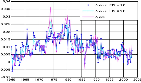
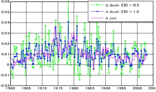
Figures 2 and 3 plot ∆coli and ∆dcolis. The property in (26) that ∆dcoli converges to ∆coli as the EIS becomes larger is confirmed in the figures. Since it might be difficult to see the differences between the COLI and DCOLIs in these figures, in Figure 4, we also plot the three-years moving averages of ∆coli, ∆dcoli, and ∆rdcoli (EIS = 0.5), which is calculated as the three-years details, see Appendix A.4.1.

6_{Note that although the shape of fluctuations in wcinverts at ψ = 1.0 (atψ = 1.0,}

wc becomes constant), the shape of the fluctuation in demeaned rdcoli (i.e., demeaned

average of inflation before and after the period, as in Reis (2005). During the first and second oil crises (i.e., 1973–1976 and 1977–1983), ∆rdcoli, which is equal to the difference between ∆dcoli and ∆coli, was the lowest. Based on the final remark in Section 2.4, it can be interpreted that the current prices of future consumption decreased, or in other words, future returns increased during the periods.7 _{On the other hand, ∆rdcoli reached its highest level}

around 1965 and 1985.

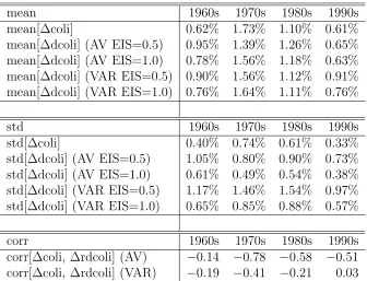
Table 1 reports the standard deviation and autocorrelation of ∆coli and ∆dcoli, and the correlation between ∆coli and ∆rdcoli.8 _{Except for the}

case where EIS = 0.2, the standard deviations of ∆dcolis are close to that of ∆coli.9 _{This is different from the results of the previous studies. The}

autocorrelation of ∆dcoli is lower than that of ∆coli. Thus, ∆dcoli is less persistent. The correlation between ∆coli and ∆rdcoli is negative. This means that when the price of current goods increases, the prices of future goods decrease, or, in other words, expected future returns increase.

In order to consider how the result is affected by human wealth, we also calculate two types of ∆dcoli that use data on households’ financial wealth instead of total wealth (we refer to them as financial ∆dcolis). One is the ∆dcoli that is calculated by (15) using the price-dividend ratio data of house-holds’ financial wealth instead of the wealth-consumption ratio.10 _{Note that}

7_{During the same periods, equity prices were relatively low.}

8_{We also calculate the average and standard deviation of ∆coli and ∆dcoli, and the}

correlation between ∆coli and ∆rdcoli for every ten years in Table 6.

9_{In the table, when EIS ≥ 1.0 (EIS = 1.0 corresponds to the log utility case), the}

volatility of ∆dcoli is less than that of ∆coli. This is because the covariance between ∆colit and ∆rdcolit is negative (note that var(∆dcolit) = var(∆colit) + var(∆rdcolit) +

2 cov(∆colit,∆rdcolit) and that corr(∆colit,∆rdcolit) is negative in the data). 10

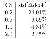
because the data price-dividend ratio does not become constant at EIS = 1.0 (log utility case), it cannot be calculated at this EIS value. The other fi-nancial ∆dcoli is calculated using dividend growth rates on fifi-nancial wealth instead of consumption growth rates in (26).11 _{Tables 2 and 3 report the}

standard deviations of the former and latter cases of financial ∆dcoli. These are highly volatile compared with the ∆dcolis that take into account human wealth. In particular, the latter financial ∆dcoli is about eight times more volatile than the ∆dcoli calculated from consumption data at an EIS of 1.0.

3.2

VAR Case

We measure the DCOLI and RDCOLI, where households (rationally) fore-cast the future using a VAR model. We assume that the expectation of a household is formed by the following VAR:

zt+1 =Azt+ϵt,

where zt is the vector of state variables, andϵt is i.i.d. with mean zero. The

components of ztare basically the same as those of Lustig and Van

Nieuwer-burgh (2006), and zt = (∆ct,∆yt, list, rta, pdat, Y Kt, rtbt, yspst)′, where ∆ct

is the per capita real consumption growth, ∆yt is the per capita real la-bor income growth, list is the labor income share, ra

t is the real return on

households’ financial wealth,pda

t is the log price-dividend ratio of households’

financial wealth, Y Kt is the output-(physical) capital ratio, rtbt is the

rela-11_{We assume that the expected values of future dividend growth rates coincide with the}

tive T-bill return, and yspst are yield spreads of several bonds. For details regarding these data, see the Appendix. We include real return rat, because

the return is related to consumption growth ∆ctthrough the Euler equation.

We also include Y Kt, because Y Kt times capital intensity is the return on aggregate capital under the Cobb-Douglas aggregate production function. Then, for example,

Et[∆ct+j] =Et[e1zt+j] =e1Ajzt,

where e1 = (1,0, . . . ,0). Matrix A is estimated from data using ordinary

least squares (OLS).

Figure 5 plots the demeaned rdcoli. Compared with the actual values case, different values of the rdcoli are observed after 2000. After 2000, the demeaned rdcoli of the VAR case is higher than that of the actual values case. This difference might be because in the actual values case, we assume that after 2003, the expected consumption growth rate is equal to the average growth rate of consumption over the sample periods.

∆coli and ∆dcoli, and the correlation between ∆coli and ∆rdcoli.12 _The

volatilities of VAR ∆dcolis are more volatile but still close to those in the actual values case.13 _{The properties on the low persistency of ∆dcoli and}

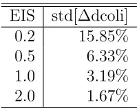
negative correlation between ∆coli and ∆rdcoli are the same as those in the actual values case. As in the actual values case, we compare these ∆dcolis with financial wealth versions of ∆dcoli. The standard deviation of finan-cial ∆dcoli consisting of the price-dividend ratio data of finanfinan-cial wealth is reported in Table 2 and that of another financial ∆dcoli calculated from ex-pected dividend growth rates is reported in Table 5.14 _{The latter financial}

∆dcolis are less volatile than the actual values version. Nonetheless, ∆dcolis calculated from expected consumption growth rates are less volatile than the latter financial ∆dcolis (the latter VAR version of financial ∆dcoli is around four times more volatile than our ∆dcoli at an EIS of 1.0).

4

Concluding Remarks

This paper develops a practical method to construct the DCOLI from con-sumption data, and using this method, measures the DCOLI. Compared with previous studies, our method has three advantages: (1) our DCOLI can

12_{As in the actual values case, we calculate the average and standard deviation of ∆coli}

and ∆dcoli, and the correlation between ∆coli and ∆rdcoli for every ten years in Table 6.

13_{The standard deviations are on average about 30% higher than those of the actual}

values case.

14_{The expected dividend growth rate is calculated by using the following relation:}

Et[∆dt+j] = (e4+e5)Ajzt−ρ−1e5Aj−1zt,

where ∆dt+jis the dividend growth rate, andeiis a row vector withi-th element unity and

other elements being zero. This relation holds becausera

t+j = ∆dt+j+pdat+j−ρ− 1

pda t+j−1

References

Alchian, Armen A. and Benjamin Klein (1973) “On a Correct Measure of Inflation”,Journal of Money, Credit and Banking, Vol. 5, No. 1, pp. 173– 91.

Bansal, Ravi and Amir Yaron (2004) “Risks for the Long Run: A Potential Resolution of Asset Pricing Puzzles”, Journal of Finance, Vol. 59, No. 4, pp. 1481–1509.

Braun, R. Anton, Julen Esteban-Pretel, Toshihiro Okada, and Nao Sudou (2006) “A Comparison of the Japanese and U.S. Business Cycles”, Japan and the World Economy, Vol. 18, No. 4, pp. 441–463.

Bryan, Michael F., Stephen G. Cecchetti, and Roisin O’Sullivan (2001) “As-set Prices in the Measurement of Inflation”, De Economist, Vol. 149, No. 4, pp. 405–431.

Bureau of Labor Statistics (2007) “The Consumer Price In-dex”, in BLS Handbook of Methods, Chap. 17. Available at http://www.bls.gov/opub/hom/pdf/homch17.pdf.

Campbell, John Y. (1993) “Intertemporal Asset Pricing without Consump-tion Data”,American Economic Review, Vol. 83, No. 3, pp. 487–512.

(1996) “Understanding Risk and Return”, Journal of Political Econ-omy, Vol. 104, No. 2, pp. 298–345.

and the Temporal Behavior of Consumption and Asset Returns: An Em-pirical Analysis”,Journal of Political Economy, Vol. 99, No. 2, pp. 263–86. Jagannathan, Ravi and Zhenyu Wang (1996) “The Conditional CAPM and the Cross-Section of Expected Returns”,Journal of Finance, Vol. 51, No. 1, pp. 3–53.

Lettau, Martin and Sydney Ludvigson (2001) “Consumption, Aggregate Wealth, and Expected Stock Returns”, Journal of Finance, Vol. 56, No. 3, pp. 815–849.

Lustig, Hanno and Stijn Van Nieuwerburgh (2006) “The Returns on Human Capital: Good News on Wall Street is Bad News on Main Street”,Review of Financial Studies, p. hhl035.

Lustig, Hanno, Stijn Van Nieuwerburgh, and Adrien Verdelhan (2008) “The Wealth-Consumption Ratio”, NBER Working Papers 13896, National Bu-reau of Economic Research, Inc.

Pollak, Robert Andrew (1975) “The Intertemporal Cost-of-Living Index”,

Annals of Economic and Social Management, Vol. 4, No. 1, pp. 179–195. Prescott, Edward C., Alexander Ueberfeldt, and Simona Cociuba (2005)

“U.S. Hours and Productivity Behavior Using CPS Hours Worked Data: 1959-I to 2004-IV”. Manuscript, Federal Reserve Bank of Minneapolis. Reis, Ricardo (2005) “A Cost-of-Living Dynamic Price Index, with an

Shibuya, Hiroshi (1992) “Dynamic Equilibrium Price Index: Asset Prices and Inflation”,Monetary and Economic Studies, Vol. 10, No. 1, pp. 95–109. Shiratsuka, Shigenori (1999) “Asset Price Fluctuation and Price Indices”,

A

Data Appendix

This appendix describes the data sources. We use quarterly data and the sample periods are 1959:4 to 2003:1.

A.1

Population and per capita hours worked

We take the working-age population (16–64 years old) and per capita hours worked data from Prescott et al. (2005).

A.2

Consumption

A.2.1 COLI

We construct Fisher’s version of COLI (or, in other words, CPI) using the formula

√ ∑

PtQt−1 ∑

Pt−1Qt−1 √

∑

PtQt

∑

Pt−1Qt

.

We chain the indices to derive the price level of consumption. To construct the indices, we use the price data of “nondurable goods” (line 6) and “ser-vices” (line 13) in Table 2.3.4 and their quantity data in Table 2.3.3 in the National Income and Product Accounts (NIPA).

A.2.2 Per capita real consumption

Nominal consumption data are from Table 2.3.5 in the NIPA. Our nominal consumption data are the sum of nondurable goods (line 6) and services (line 13). These data are seasonally adjusted at annual rates. Thus, we divide the values by 4.

A.3

Labor income

A.3.1 Labor income share

Data on labor income share are taken from Table 2.1 in the NIPA. The labor income share is calculated by the nominal labor income explained below /

nominal “disposable personal income” (line 26).

We construct nominal labor income from “compensation of employees, received” (line 2) + “government social benefits to persons” (line 17) −

“contributions for government social insurance” (line 24) − labor taxes. As in Lettau and Ludvigson (2001), the labor taxes are imputed from the labor tax ratio×the nominal labor income, where the labor tax ratio is calculated as the ratio of “wage and salary disbursements” (line 3) to “wage and salary disbursements” + “proprietors’ income with inventory valuation and capital consumption adjustments” (line 9) + “rental income of persons with capital consumption adjustment” (line 12) + “personal income receipts on assets” (line 13).

A.3.2 Per capita real labor income

× real disposable personal income. The real disposable personal income is obtained by “disposable personal income” (line 26) / the COLI explained above.15 _{In order to obtain the per capita real labor income, we divide it}

by the population explained above. These data are seasonally adjusted at annual rates. Thus, we divide the values by 4.

A.4

Households’ financial wealth

A.4.1 Price-dividend ratio of households’ financial wealth pda

In order to obtain the price-dividend ratio of households’ financial wealth,

pda_{, we divide the nominal financial wealth by nominal dividends minus}

savings, both of which are explained below.

Nominal financial wealth data are obtained from the balance sheet of households and non-profit organizations, Flow of Funds Accounts Table B-100, provided by the Federal Reserve Board System. This wealth measure is on an end-of-period basis. Therefore, we use the t−1 value of the data for period t wealth. Our measure of households’ financial wealth consists of net worth (line 41)−consumer durable goods (line 7). Basically, our definition of nominal financial wealth is the same as that of Lettau and Ludvigson (2001) except that we exclude durable consumption from nominal financial wealth (because we exclude durable consumption from our consumption data).

Nominal dividends minus savings are obtained from Table 2.1 in the NIPA. It is constructed by “proprietors’ income with inventory valuation and capital consumption adjustments” (line 9) + “rental income of persons

15

with capital consumption adjustment” (line 12) + “personal income receipts on assets” (line 13) − “other current transfer receipts, from business (net)” (line 23) − capital taxes − “personal saving” (line 33). Similar to the la-bor taxes above, the capital taxes are imputed from capital tax ratio ×

the nominal capital income, where the capital tax ratio is calculated as the ratio of “proprietors’ income with inventory valuation and capital consump-tion adjustments” + “rental income of persons with capital consumpconsump-tion adjustment” + “personal income receipts on assets” to “wage and salary dis-bursements” (line 3) + “proprietors’ income with inventory valuation and capital consumption adjustments” + “rental income of persons with capital consumption adjustment” + “personal income receipts on assets.”

A.4.2 Real return of households’ financial wealth ra

We obtain the real return on households’ financial wealth, ra _{from r}a t+1 ≡

lnRt+1 = ln(

Pa t+1

Pa

t−Dat), where P

a _{is the per capita real financial wealth, and} Da _{is the per capita real dividends minus savings. P}a _{is calculated from the}

nominal financial wealth explained above divided by the COLI and popula-tion. Da _{is calculated from nominal dividends minus savings divided by the}

COLI and population.

A.5

Relative T-bill return

rtb

and yield spreads

ysps

Relative T-bill return rtbt and the yield spreads of several bondsyspst used in the VAR case are taken from Van Nieuwerburgh’s website. Precisely, rtbt

lefsprBaaT-bond, and termspread in quarterly_data_WSMS.xlson his website.

A.6

Output-(physical) capital ratio

Y K

std[∆coli] AC(1)[∆coli] AC(4)[∆coli] AC(8)[∆coli] 0.71% 0.82 0.63 0.37

EIS std[∆dcoli] AC(1)[∆dcoli] AC(4)[∆dcoli] AC(8)[∆dcoli] corr[∆coli,∆rdcoli] 0.2 2.35% 0.21 0.02 −0.16 −0.52

0.5 0.91% 0.27 0.09 0.01 –

1.0 0.62% 0.61 0.44 0.36 –

2.0 0.61% 0.81 0.64 0.47 –

Table 1: Standard deviation and autocorrelation of ∆coli and ∆dcoli, and correlation between ∆coli and ∆rdcoli of the actual values case. Notes: AC(d) represents the autocorrelation ofd lags. corr[∆coli,∆rdcoli] does not depend on the EIS value.

EIS std[∆dcoli] 0.2 6.47% 0.5 10.34% 1.0 n.a. 2.0 5.28%

Table 2: Standard deviation of the financial ∆dcoli calculated using the price-dividend ratio data of broad financial wealth instead of the wealth-consumption ratio. Note: For details regarding the price-dividend ratio data, see appendix A.4.1.

EIS std[∆dcoli] 0.2 24.01% 0.5 9.59% 1.0 4.81% 2.0 2.45%

EIS std[∆dcoli] AC(1)[∆dcoli] AC(4)[∆dcoli] AC(8)[∆dcoli] corr[∆coli,∆rdcoli] 0.2 3.16% 0.06 −0.05 −0.14 −0.29

0.5 1.30% 0.07 −0.02 −0.11 –

1.0 0.81% 0.31 0.21 0.06 –

2.0 0.69% 0.62 0.48 0.26 –

Table 4: Standard deviation and autocorrelation of ∆dcoli and correlation between ∆coli and ∆rdcoli of the VAR case. Notes: AC(d) represents the autocorrelation of d lags. corr[∆coli,∆rdcoli] does not depend on the EIS value.

EIS std[∆dcoli] 0.2 15.85% 0.5 6.33% 1.0 3.19% 2.0 1.67%

Figure 1: Demeaned rdcolis of the actual values case.

Figure 2: ∆coli and ∆dcolis (for DCOLI, EIS = 0.2 and 0.5) of the actual values case

Figure 4: Three-years moving average of ∆coli, ∆dcoli, and ∆rdcoli (for ∆dcoli and ∆rdcoli, EIS = 0.5) of the actual values case

Figure 5: Demeaned rdcolis of the VAR case