Munich Personal RePEc Archive
SHOULD THE UTILITY FUNCTION
BE DITCHED?
Dominique, C-Rene
27 November 2007
Online at
https://mpra.ub.uni-muenchen.de/5987/
SHOULD THE UTILITY FUNCTION BE DITCHED?
C-René Dominique
ABSTRACT
This note takes a retrospective look at the Utility Construct still in use in economic science and compares it to a new approach based on recent findings in neuroscience. The results show that it is more natural and more compelling to go from the preference order to the price vector. Thus making the non-falsifiable utility apparatus superfluous.
I- INTRODUCTION
A C2 function is one whose second derivatives in its arguments exist and are
continuous. According to a group of economist-pioneers, a throw-off of some individual’s
C2 utility function is a well-defined demand function, which is differentiable and
homogeneous of degree zero in budget and prices, a corner stone of economic theory. The
utility function itself is supposedly derived from a well-ordered individual preference
relation, thus making the demand function dependent on two subjective concepts; namely, a
C2 utility function and a well-ordered preference relation. The economizing problem is
essentially one of optimization, but the early pioneers were not sure as to how to proceed to
optimization from a mere ranking, whether well-ordered or not. In addition, it was initially
and erroneously believed that utility maximization would yield richness and robustness;
hence the foray into utility, as preference was debased to a primitive concept.
However, the path from a well-ordered preference relation to a C2 function is fraught
with some dangerous anomalies. Initially, it was thought that a strictly convex and
continuous preference relation suffices to yield a strictly quasi-concave utility function.
Subsequently, however, it was realized that these properties might not have been strong
enough to yield an everywhere differentiable demand function. Additional conditions would
be required at the levels of both preference and utility. That realization spurred the vast
research programme that gives substance to today’s economists’ discourse on utility. In
and time to figure out all conditions they thought were necessary to arrive at well-specified
demand functions. The relevant and voluminous literature attests to that. See for example,
Pareto (1896), Wold (1943, 1944), Samuelson (1947), Debreu (1959, 1960, 1964, 1976),
Radner (1963), Sonnenschein (1965, 1971), Smeidler (1971), Koopmans (1972),
Hildenbrand (1974), Shafer (1974), just to name a few. However, despite that effort, the
preference order-utility construct remains to this day hazy and problematic. Worst still, its
predictions are regularly falsified whether in simple observation, personal experience, or in
experimental designs.
At first sight, one would think that economists should be uneasy when faced with
such incongruities, but one should also bear in mind that when these concepts were being
developed, they had no means of gazing into the workings of the human brain. This is no
longer so, however. With more mature reflections and new tools(1) (developed by
physicists), neuroscientists are now able to examine the brain’s architecture in a non
invasive manner. Their findings are compelling enough to encourage economists to revisit
their construct; and this note is a first step in that direction.
I will first briefly review the existing construct mainly to see why the ensuing
problems continue to defy satisfactory solutions. Next, I will examine an alternative
approach based on the findings of neuroscience, and compare the two sets of results. As the
results of the alternative approach are very compelling, hopefully, they might sway
economists to finally view the utility function as an unnecessary appendage.
II- CONDITIONS FOR A WELL-ORDERED PREFERENCE RELATION
Until the late 1920s, the notion of preference relation was loosely equated with utility.
At the same time though, many were still confusing preference with taste, which was
thought to be fixed. Around the 1940s, however, economists began to differentiate the two.
While recognizing preference as more basic, utility began to appear as a more convenient
device to describe consumer behavior; although nobody knew how preferences were
formed, and to this day it seems that whatever is said about preferences still leaves the
associated utility function incompletely specified. To avoid pathologies, therefore,
economists began to ‘finick’ both concepts so as to meet the requirements of maximizing
rules to undertake the task with thoroughness. For tractability, I show in Table 1 a list of
axioms and conditions that the preference relation is supposed to satisfy and to which I will
refer throughout the discussion. To arrive at a C2 utility function, still more are needed, but
I will only mention them only in passing, because they will not be necessary for the present
purpose. In fact, I believe that that additional panoply of conditions is outright superfluous.
For in this case, mathematical formalism, though helpful in description and analysis, can
not dictate consumer behavior. Further, to describe, mathematically or otherwise, one must
first understand, although but in the present case, it seems that formalism had taken
precedence over concreteness.
Imaging a typical consumer, denoted by i, facing consumption set X, which a
collection of consumption bundles as its elements. In general, X is the non negative orthant
in Rk+ (k =1, 2, …,n), where R is the reals. For ease of exposition, however, I posit X = {x,
y, z}, where x, y, and z are thing-like entities over which consumer i expresses a value
judgement at a particular instant of time. A binary relation P on X is a subset of the
Cartesian product on X with itself. Also P stands for a weak preference. Thus writing (xPy)
means that x is preferred to y, because consumer i considers x ‘as good as’ y. The binary
relation becomes an equivalence relation, I, under certain conditions, in the sense that
writing (xIy) means that i is ‘indifferent’ between x and y; in other words, (xIy) if and only
if (xPy) and (yPx), implying the symmetry of I.
Still later on, economists realized that a weak preference relation could not ensure
continuity in P, hence, nor in u(.), the utility function, because the upper and lower contour
sets of P are ‘closed’ relative to X. They then posited P’ as a strict preference relation (a
stronger assumption). Thus (xP’y) means that x is ‘strictly preferred to’ y, because i
believes that x is ‘as good as’ y, but not conversely. The supposed advantage here is that
under P’, the upper and lower contour sets are ‘open’ relative to X.
Referring to Table 1, a P’ that meets A1-A4 and C1 is said to be linear or complete.
The equivalence relation satisfying B1-B3 follows. Monotonicity (C2) too follows
naturally for most goods. Thus, the difference between P and P’ is reduced to the
following: P satisfies A3, A4 and B1, while the indifference relation given by,
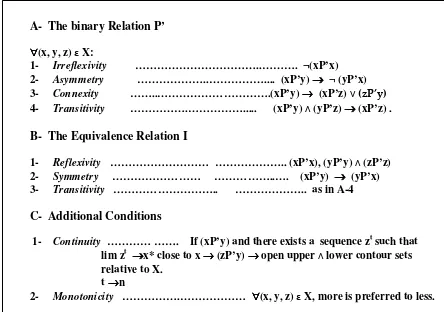
TABLE 1: Axioms and conditions* for a Well-Ordered Preference Relation
i., e., the intersection of the contour sets are closed under P and open under P’. It can
immediately be seen why P’ does not admit B1, for, x, say, cannot be strictly preferred to
itself. However, this difference is a consequence of C1 that ensures continuity and which at
once seems to introduce surreptitiously time in the analysis. In words, C1 says that if
(xP’y), say, and if there exits a sequence zt that converges to some x* close to the bundle x,
then (zP’y). Then, it is not farfetched to assume that the consumer can order X in time, as
the sequence converges in finite time. If z1, z 2, z 3 , … are subsequent selections, then there
is a time dimension, which somehow had gotten lost in the analysis; I will later return the
question of time and to other questions relative to the empirical content of A4. For the time
being, let us suppose that if P’ satisfies A1- A4 and C1, the relation I will satisfy B1-B3.
Then P’ is said to be linear or complete. We may also call it an ‘empirical relational
system’, represented by: X, P’, I . To justify that claim and to say more about it, Theorem
1 may be invoked:
A- The binary Relation P’
∀ ∀∀
∀(x, y, z) ε X:
1- Irreflexivity ………..………. ¬(xP’x) 2- Asymmetry ………..……….... (xP’y) →→→→ ¬ (yP’x) 3- Connexity ……..……….(xP’y) →→→→ (xP’z) ∨ (zP’y)
4- Transitivity ……….………... (xP’y) ∧ (yP’z) →→→→ (xP’z) .
B- The Equivalence Relation I
1- Reflexivity ……… ……….. (xP’x), (yP’y) ∧ (zP’z) 2- Symmetry ……… ………..…. (xP’y) →→→→ (yP’x) 3- Transitivity ……….. ……….. as in A-4
C- Additional Conditions
1- Continuity ………… ……. If (xP’y) and there exists a sequence zt such that lim zt →→→→x* close to x →→→→ (zP’y) →→→→ open upper ∧ lower contour sets relative to X.
t →→→→n
Theorem 1 If X, P’, I is linear or complete, then it has a countable base and it can be represented by an ordinal one-dimensional scale.
Next, Zorn’s Lemma (1935) can be also be invoked to justify the following consequential statements (CT):
CT-1 An ordered set, X, is said to be well-ordered if X and each of its non-empty
subsets have first elements in the prescribed ordering of X.
CT-2 Every well-ordered set X is totally ordered.
CT-3 The converse of CT-2 holds if X is finite.
This result is upheld as significant and it authorizes its authors to claim that if X, P’, I is
well-ordered, then there exists a continuous utility function u: Rk+→ R+. Furthermore, if u
and u’ are both maps of the empirical relational system X, P’, I into a real number R, then
u’ is a monotone transformation of u.
At this juncture, it might be of interest to stress once more that P’ is selected over P,
because the latter, although more basic, was thought to be unable to meet all the associated
topological conditions to generate a well-defined u. Can P’ do so? Not quite. The
consumption sets of the poor are difficult to well-order due to product differentiation (i., e.,
lack of information). The consumption sets of non-poor (most consumers) consist of
necessities and discretionary goods. That is, those two types of goods are not really
comparable. In such a case, the continuity assumption (C1) is violated. Only a lexicographic
order is possible, as trade-offs between necessities and discretionary goods do not exist.
Indeed, the very definition of the binary relation is not satisfied. The monotonicity
assumption is satisfied in most cases; that is, when the entities are thing-likes, but not
generally as in the case of leisure, for example, where less may be preferred to more. More
telling though is that consumers continue to make intransitive choices, and sometime they
are observed even acting in a manner that seems contrary to the dictates of utility
maximization. Following that another debate ensued. Sonnenschein (1965) argued that
continuity (C1) and connexity (A3) suffice to ensure transitivity (A4). Shafer (1971)
followed, arguing that continuity and transitivity just imply connexity. But again, many
known relations simply do not display continuity as in the case of lexicographic ordering.
conditions such as convexity, upper-semi-continuity, indirectness, separability,
Cobb-Douglas-ness, etc. in an attempt to bloc eventual anomalies. As a result, instead of the
ordinal scale allowed by Theorem 1, they have inadvertently produced a theoretically safe
construct, also one that has been proven not to have any empirical content.
III- AN ALTERNATIVE
I have given the reader a succinct account of why these early pioneers were so eager
to construct a C2 utility function. One can easily understand that, knowing preciously little
about how preference was formed, they had to rely on Boolean reasoning and operations to
grapple with the slipperiness of such a concept. More recently, however, new tools have
been made available. Now neuroscientists can readily observe brains’ workings easily and
non-intrusively(2). As a result, the brain comes to be viewed as essentially a dynamic
input/output structure. Mathematically and succinctly put, there exist a set of external input
stimuli, satellite structures (such as the visual cortex), two state spaces, (L) and (χ), and a
number of maps. L is the limbic system or the brain stem, χ is the frontal cortex, some of
the maps are ‘onto’ while others are ‘one-to-one’. Moreover, L is the site of memory
(factual and emotive experience), and χ is where computation, deduction and overall
evaluation take place.
To clarify, consider an example of how external stimuli are mapped onto L, and χ.
Seeing a bundle x, say, means that light patterns are received in the photoreceptor cells in
the retina, where they are immediately converted into neuronal signals, and the
neurotransmitter acetylcholine is released throughout the prefrontal cortex and to all its
satellite structures (Crick and Koch, 2003; Koch, 2007). This gives rise to an emergent
property, e, which focuses and directs attention to a task, implying also that the seer is in
the state of wakefulness (Greenfield, 2007). Next, neuronal signals, made out of
specialized neurons, traveled through the optic nerve to the lateral geniculate nucleus in the
thalamus, and from there to the visual cortex (where light patterns are identified) via the
neural cords (called optic radiation, leading to the occipital lobe) and on to the
hippocampus (Martinez-Conde, 2006; Martinez-Conde and Macknik,2007). The later
invariantly organized hierarchically from the general to the specific (Tsien, 2007).
Different cliques or circuits respond to perceptual, factual and emotional aspects of the
inputs. Beside, the hippocampus receives information from photoreceptors, from the
geniculate nucleus, from the vestibular system, from the locus coerulus, from the amygdala,
etc. and from other neurons encoded with general and abstract information to be used in
future situations. Thus, the identification of x fed to χ by L and other satellite structures for
a final evaluation is a mixture of factual and emotional assessments of the image of x or
something likes it. This complex flows may be conveniently divided into two categories,
namely objective information, I0, and the emotive mixture, eL. Therefore, state space χ may
be represented by a dynamical system I0, eL, e that brings these two flows of
neurotransmitters into an equilibrium; that equilibrium is of course, an informational
equilibrium, but it is similar to a thermodynamic one.
In all of this, the role of the emergent factor, e ε [-1 1] can not be overemphasized. It
exists only in the state of wakefulness (compared to the state of dormancy); it is the maestro
in charge of the traffic of neurotransmitters from various parts of the brain; it may be
associated with judgement and its intensity varies with the intensity of the input stimulus
(Greenfield, 2007). If the informational assessment realized in state space χ is a ‘scalar
field’, then e gives the field a direction.
I have shown elsewhere (Dominique, 2006), that the assessment of the state space χ is
none other than a “potential” that must be minimized using a differential map. It suffices
for the present purpose to say that the equilibrium value, P, is some sort of a linear
combination of I0 and eL. The stronger are the intensities of these flows the higher is P.
With an appropriate additional transformation, I was able to identify the topology of the
brain as a bi-modal cusp catastrophe given by:
(i) Ψ( I0, eL, e ) ε C∞ (Rv + c, R),
where v ≤ 2 is the corank and c is the codim of Ψ. To put it differently, the two ordinal
scales in χ are mapped onto two equilibrium manifolds, M+ and M-. M+ maps equilibrium
points onto R+ and, analogously, M- maps equilibria onto R-.
In the present case, appealing to the Thom’s (1975) Classification Theorem proved
neuroscientists affirm that signals travel at speed up to 525 feet a second, I then ignored
slow dynamics to concentrate on points mapped onto R+ under very fast dynamics. When
they are projected onto R+, such points are not equidistant near the maximal element (the
highest point in the direction in which preference runs) as the equilibrium manifold is a
curved surface. Hence, preference indices near but inferior to the maximal element are
more compact, while those near but superior to the minimal element are more unclenched.
This means that the continuity property of P is not guaranteed. Finally, it can immediately
be seen that the manner in which all additional or new information are appraised in χ may
shift an equilibrium point on M+ or may even cause it to jump onto M- ; implying that it is
possible to go from preference to dis-preference in a natural way.
If equilibria are given by P, and the well-ordered preference is denoted Rxyz, solving
the economizing problem implies applying the maps Ð, h1, h2 and M. That is, Ð: I0, eL, e
→ , h2: → Rxyz, such that:
(ii) M = Rxyz → P,
where M, is a composite map or a market (simplified to a pure exchange) that takes us to
the price vector P directly from the ordering.
The way M is constructed is as follows: First, it ignores points on M-, as goods
eliciting such equilibria are not in the consumption set X. Suppose consumers are limited
to 3 (i =1,2, 3), then Px , Py, Pz, mapped onto R+ yield the ordering (xP’y) ∧ (yP’z), call it
ℜi . In equilibrium, that ordering is preserved when it is mapped onto market shares, ∝,
and onto total equilibrium expenditures (∝B). Since in equilibrium, expenditures are equal
to market values (V), then, we have:
ℜixyz →Vx >Vy> Vz = (∝ixBi)>(∝iyBi)>(∝izBi). If Vx = (∝ixBi) →∆Px /∆x< 0,∀(x,y,z)εX.
If now ℜixyz is mapped onto the budget share set {∝i } such that i∝xyz = 1, and if supply is
fixed, then in equilibrium:
i∝xi > i∝yi > i∝zi → Px > Py > Pz .
Thus, the utility construct is unnecessary, and there is no explicit effort on the part of the
IV-FINAL REMARKS
I have tried to show that Theorem 1 allows for a simple ordinal scale:
(iii) u ( X, P’, I) : Rk → R+ ,
as equation (iii) does not completely specify u(.). But to satisfy the imperative of utility
maximization, economists construct:
(iv) u ( X, P’, I ) ε C2 (Rk , R+);
this produces uncomfortable anomalies. By integrating the findings of neuroscience, we
arrive at equation (ii) above, which is more concrete and presents a number of advantages
over the conventional one. To wit:
Firstly, it dispenses with the need of continuous ordinal scales in conformity with
nature itself, which is not continuous. Secondly, it is robust to a violation of the
monotonicity condition, because it accounts for the context; thing-like objects are special
cases. Thirdly, it distinguishes between transitivity and ambivalence. In this alternative,
transitivity occurs when two imperfect substitute bundles receive the same ranking; the
information set of the consumer is considered (by him or her) complete and, therefore, there
is no reason for the consumer to appear inconsistent. Ambivalence, on the other hand, may
occur when the substitutes have different attractive characteristics, but the information set is
incomplete; in that case, the consumer can not decide on the ranking. Fourthly, it gives
substance to what Simon (1985) has termed ‘objective’ and ‘subjective’ rationalities; here,
they appear as a linear combination. Fifthly, it resolves the dilemma of the so-called called
Ultimatum Game(3). That is, the proportion offered to player B might be deemed unfair
and, therefore, B turns it down to punish greed; in such a case, the flow eL dominates I0.
Sixthly, it resolves a phenomenon observed by Tversky and Kaneman(4) (1981). That is, by
letting x stands for money, and y for theater ticket, we have: (yP’x) in state 1, and (xP’y) in
state 2; this is explained by what philosophers call ‘change in preference horizon’ or
‘different states of nature’ by economists. Seventhly, the conventional presentation can not
explain changes over time in the utility function; here the time element is ever present.
Eighthly, the conventional approach can not accommodate the impacts of emotions on
etc... Frank Knight, for example, believed that “human activity is largely impulsive
response to stimuli and suggestions.”
Finally, it should be observed that an equilibrium point mapped onto R+ is a
valuation, V. The higher is the position of x in the ranking, the higher is the V of x,
commanding a corresponding proportion ∝ of consumer i’s budget B. Hence, if both
quantity and price could be made perfectly divisible, individual consumer demand could be
a rectangular hyperbola. Indeed, in Dominique (1999, ch.3), it is shown how the invertible
map M is constructed for a simple 3 goods-3 consumer economy to minimize a potential
market gain, and how it easily maps ℜ onto P (the equilibrium price vector of a pure
exchange model), but without the hypothesis of utility maximization. And variations in the
price vector are perfectly correlated with changes in the ranking order.
NOTES
1 For example, Computed tomography scans (CT), Positron Emission tomography scans (PET), Magnetic Resonance Imaging (MRI), Functional Magnetic Imaging (fMRI), Magneto-encephalography (MEG), Trans-cranial Stimulation (TMS), etc.
2 Many of their findings are discussed in the popular press. See, for example, The New York Times, June 17, 2006, and November 22, 2006, US& World Report, Oct. 18, 2006, and Scientific American, July, August and October 2007.
3 This experiment involves two players, A and B. A, say, is given a certain sum, s, and A must give a proportion k of his or her choosing to B. If B accepts k s, then B may keep (1-k) s. However, if A refuses k s, as she deems k too low, both players end up with nothing. The experiment shows that if k is less than 20 percent of s, the offer is rejected.
4 Tversky and Kaneman have observed that 88 percent of subjects in their sample say if they arrived at a theater to buy a $ 10 ticket for a play and then discovered that they had lost $10 on the way, they would buy the ticket anyway. But if the ticket was bought in advance and discovered when they arrived in the theater that they had lost the ticket, 54 percent say they would not buy another ticket. In the conventional approach, the 54 percent would be labeled ‘irrational’.
REFERENCES
Crick, F. and Koch, C. (2003). “A Framework for Consciousness.” Nature Neuroscience,
vol.6, 119-126.
---(1960) “Topological Methods in Cardinal Utility Theory” in K. J. Arrow, et al.
(eds). Mathematical Methods in Social Sciences. Stanford: Stanford Univ. Press,
1960.
---(1964) “Continuity Properties of Paretian Utility.” International Economic
Review, vol. 5, 285-293.
---(1976) “Smooth Preferences. A Corrigendum.” Econometrica, vol. 44,
831-832.
Dominique, C-R. (1999). Unfettered Globalization. New York: Praeger/Greenwood Pub.
---(2006). “Explaining the Logic of Pure Preference in a Neurodynamic Structure.” MPRA Paper no. 3, Univ. Library of Munich, Germany. See also
http:/Logec.Repec.org / RAS / pdo127. htm; www .harin. info.
Greenfield, S. A. and Collins, T. E. (2005). “A Neuroscientific Approach to
Consciousness.” Progress in Brain’s Research, vol. 150, 11-23.
---(2007). “How Does Consciousness Happen?” Scientific Amer. October, 76-83.
Hildenbrand, W. (1974). Core and Equilibria of a Large Economy. Princeton: Princeton
Univ. Press.
Koch, C. (2007). “How Does Consciousness Happen?” Scientific Amer., October, 79.
Koopmans, T (1972). “Representation of Preference Ordering With Independent
Components of Consumption.” in C. B. McGuire and R. Radner (eds). Decision and
Organization. Amsterdam: North-Holland, 1972, 57-78.
Lin, L. et al. (2005). “Identification of Network Level Coding Units for Real-Time
Representation of Episodic Experience in the Hippocampus.” Proceedings of the
National Academy of Sciences, vol. 102, 6125-6130.
---(2006). “Organizing Principles of Real-Time Memory Encoding.” Trends in
Neuroscience, vol. 29, 48-57.
Martinez-Conde, S. et al. (2004). “The Role of Fixational Movements in Visual
Perception.” Nature Review Neuroscience, vol. 5, 229-240.
Martinez-Conde, S. and Macknik, S. (2007). “Windows on the Mind.” Scientific Amer.,
Aug.56-63.
Pareto, V. (1896). Cours d’économie Politique. Lausanne: Rouge.
Radner, T. (1963). “The Existence of a Utility Function to Represent Preferences.” Review
of Economic Studies, vol. 30, 229-232.
Samuelson, P. A. (1947). “Some Implications of Linearity.” Review of Economic Studies,
Shafer, W. J. (1974). “The Nontransitive Consumer.” Econometrica, vol.42, 913-919.
Simon, H. (1985). “Human Nature in Politics: The Dialogue of Psychology and Political
Science.” Amer. Pol.Sc.Rev., vol. 79, 293-304.
Smeidler, D. (1971). “A Condition for the Completeness of Partial Preference Relations.” Econometrica, vol. 39, 403-404.
Sonnenschein, H. (1965). “The Relationship Between Transitive Preference and the
Structure of the Choice Space.” Econometrica, vol. 33, 624-634.
---(1971). “Demand Theory Without Transitive Preferences.” In J. S. Chipman et
al. (eds) Preference, Utility and Demand. New York: Harcourt Brace Jovanovich.
Thom, R. (1975). Structural Stability and Morphogenesis. Reading, MA: Benjamin.
Tsien, J. Z. (2007). “The Memory Code.” Scientific Amer. July, 52-59.
Tversky, A. and Kaneman, D. (1985). “The Framing of Decisions and the Psychology of
Choice.” Science, vol.211, 435-458.
Wold, H. O. (1943). “ A Synthesis of Pure Demand Analysis.” Skandinavisk
Aktuarietidskrift vol. 26, 85-118.
---(1944). “A Synthesis of Pure Demand Analysis.” Skandinavisk Aktuarietdskrift,
vol. 27, 69-120.
Zorn, M. (1935). “A Remark on Method in Transfinite Algebra.” Bull. Amer.Mathematical
Soc., vol.41, 667-670.