A Heuristic Model for Tasks Scheduling in
Heterogeneous Distributed Real Time System under
Fuzzy Environment
Harendra Kumar
Department of Mathematics and Statistics
Gurkula Kangari University, Hardwar-249404, Uttarakhand (India)
ABSTRACT
The development of distributed real time system (DRTS) has lead to there use in several applications including information processing, fluid flow, weather modeling, database systems, real-time high-speed simulation of dynamical systems, and image processing. Reliability analysis of these processing elements and communication links is one of the important parameter to get the system efficiency. We can improve the system performance (i.e. system cost, system reliability and processor utilization etc.) by scheduling the tasks to the processors properly in DRTS. In this paper, a new tasks allocation model has been developed with fuzzy execution times 𝑒 𝑖,𝑗 and fuzzy inter tasks communication times 𝑐 𝑖,𝑗.The times has been defuzzified into crisp one by using Robust Ranking Method [RRM], Centre of Maxima Method [CoM] and Weight of Center of Area Method [CoA].The effect of inter processor distances on the tasks allocation has been considered while developing the model. Numerical examples show that the model presented in this paper is suitable for arbitrary number of processors with random program structure and more realistic and general in nature.
Keywords
Distributed real time systems, Fuzzy execution times, Fuzzy inter tasks communication times, Reliability.
1.
INTRODUCTION
A distributed real time system is a computing platform where hardware or software components located at networked computers communicate and coordinate their actions only by passing messages. It enables users to access services and executes applications over a heterogeneous collection of computers and networks. In a DRTS the execution of a program may be distributed among several computing e l e m e n t s to reduce the overall system cost by taking a d v a n t a g e o f heterogeneous c o m p u t a t i o n a l capabilities a n d other resources within the system. Reliability is defined in terms of the time interval in contrast to an instance in time defined in availability. A highly reliable system is one that will continue working for a long period of time. The often advocated advantage of the DRTS, in comparison to the centralized system, is the reliability due to the existence of multiple resources. However, only the multiple instances of resources cannot increase the reliability of the DRTS, rather the various processes of the distributed operating system (viz. memory manager, task scheduler etc.) must be designed properly to increase the reliability by extracting the characteristic features of the DRTS.
The module allocation in a distributed processing system finds extensive application in the faculties where large amount of data is to be processed in a short period of time or where real time computations are required. The main incentives for choosing DRTS are higher throughput,
improved availability a n d better a c c e s s to a widely communicated w e b of information. The increased commercialization o f communication s y s t e m s means that ensuring system reliability is of critical importance i n h e r e n t l y . DRTS is more complex, therefore it is very difficult to predict the performance of DRTS. Mathematical modelling is the tool which can play an important role to predict the performance of DRTS. In order to make best use of the resources, it becomes essential to maximize the overall throughput by allocating the t a s k s to processors in such a way that the allocated load on all the processors should be balanced and to minimize the inter tasks communication b y assigning tasks to same processor as much as possible. Which are both contrary t o each other as an increase in the number of processors may actually decr ease the total throughput of the system. This degradation effect is known as saturation effect, which occurs due to heavy communication traffic induced by data transfers between tasks that reside on separate processors. An allocation policy can be static or dynamic, depending upon the time at which the allocation decisions are made. In static allocation once a task is assigned to a processor, it remains there statically during the execution of a distributed program. Many approaches have been reported for solving the Static
tasks assignment problem in a DRTS [1-7]. While in dynamic allocation a module can be reassigned during program execution [8-11]. Donight et al [12] has determined the level of reliability of components with expending low cost. X. Kong et al [13], proposed an efficient dynamic task scheduling scheme for virtualized data centres. A model for allocating the tasks to processors in heterogeneous distributed computing systems with the goal of maximizing the system reliability has been developed in [14]. Kumar et al. [15] has developed a task allocation problem using fuzzy execution and fuzzy communication times. RecentlyV.Sriramdas et al [16] developed a tasks allocation model treating allocation factors as fuzzy numbers.
This paper deals with the tasks allocation problem having multiple objectives such as: minimization of system cost, maximization of system reliability and load balancing for proper utilization of the processor’s capacity. The rest paper is organized as follows. Tasks allocation problem with notations, definitions and assumptions used are defined first in section 2. In section 3, tasks allocation model has been discussed. The Section 4 shows the experimental results and section 5 concludes the paper.
2.
THE PROBLEM
An allocation of tasks to processors is defined by a function, A from the set T of tasks to the set P of processors such that: A: T→P, where A (i) = j if task ti is assigned to
Each processor has local memory only and do not share any global memory. The fuzzy execution times (FET), 𝑒 𝑖,𝑗 of the tasks on the processors is taken in the form of matrix named as fuzzy execution time matrix (FETM), 𝐹𝐸𝑇𝑀 = 𝑒 𝑖,𝑗 of order m x n. The fuzzy inter-tasks communication times (FITCT), 𝑐 𝑖,𝑗 is taken in the form of a symmetric matrix named as fuzzy inter task communication time matrix (FITCM), 𝐹𝐼𝑇𝐶𝑇𝑀 = 𝑐 𝑖,𝑗 of order m. In this paper times
𝑒 𝑖,𝑗 and 𝑐 𝑖,𝑗 have been considered to be triangular and trapezoidal numbers. In general the objective of this paper is to find an optimal allocation AO, which minimize the response
time of the program and optimize the system reliability by properly mapping the modules to the processors. In order to make the best use of the resources in a distributed computing system we would like to distribute the load on each processor in such a way that allocated load on the processors are balanced. The following notations, terms and assumptions w i l l be used throughout the text.
2.1
Notations:
P : {p1, p2, . . . , pn} is the set of
n-heterogeneous processors T : {t1, t2, . . . , tm} is the set of m-tasks
𝑒 𝑖,𝑗: Fuzzy execution time (FET) for the task ti, running on processor pj
𝑐 𝑖,𝑗: Fuzzy inter-task communication time (FITCT) between ti and tj
FETM= 𝑒 𝑖,𝑗 : Fuzzy execution time matrix
FITCTM= 𝑐 𝑖,𝑗 : Fuzzy inter-task communication time matrix
λk : Failure rate of kth processor
μkb: Failure rate of communication link (or
path) lkb between two processors pk and
pb
CLFRM=[µkb]: Communication link failure rate matrix
wkb: Transmission rate of communication link
(or path) lkb
dkb : Distance between two processor pk and pb
IPDM=[dkb]: Inter processor distance matrix
2.2
System Costs:
The fuzzy execution time 𝑒 𝑖,𝑗 is the amount of the work to be performed by the executing task ti on the processor pj. For an
allocation A, the overall fuzzy execution time and fuzzy execution time for each processor are calculated by using equations (1) and (2) respectively as:
, ( ) 1
( ) i A i
i m
FET A e
% (1), ( ) 1 ( )
j
j i A i
i m i TS
PFET A e
% ,where TSj= {i: A(i) =j, j=1, 2…n} (2)
The fuzzy inter task communication time 𝑐 𝑖,𝑗 is incurred due to the data units exchanged between the tasks ti and tj if they
are on different processors during the process of execution. Let us denote dx,y the distance between the processors Px and
Py. The processors Px and Py are connected by a
communication link say lx,y. The inter-processor
communication cost per unit of information transferred between two processors Px and Py increases linearly as the
distances dx,y increases. To consider the impact of inter
processor distance on the cost, we define a inter processor distance matrix IPDM= [dx,y]. Thus, if two interacting tasks ti and tj are assigned to two different processors Pk and
Ps respectively, then the two tasks cause the inter-processor
communication cost of 𝑐 𝑖,𝑗*dk.s.We assume that the
communication cost between two tasks assigned to the same processors is negligible, since all communication is through memory as opposed to an inter-processor link.
For an allocation A, the overall fuzzy inter-task communication times and fuzzy inter-task communication times for each processor are calculated by using equations (3) and (4) respectively as
𝐹𝐼𝑇𝐶𝑇 𝐴 = 1≤ 𝑖 ≤ 𝑚 𝑐 𝐴(𝑖),𝐴(𝑗 )∗ 𝑑𝐴 𝑖 ,𝐴(𝑗 ) 𝐼+1≤𝑗 ≤𝑀
𝐴(𝑖)≠𝐴(𝑗 )
(3)
𝑃𝐹𝐼𝑇𝐶𝑇(𝐴)𝑗 = 1≤ 𝑖 ≤ 𝑚 𝑐 𝐴(𝑖),𝐴(𝑘) 𝑖+1≤𝑗 ≤𝑚
𝐴 𝑖 =𝑗 ≠𝐴(𝑘)
(4)
The total cost, TCOST (A) of the system for an allocation A is computed as:
TCOST(A) = FET(A) +FITCT(A) (5) The response time (RT) is a function of the amount of computation to be performed by each processor and the communication time. This function is defined by considering the processor with the heaviest aggregate computation and communication loads of the processors. The fuzzy response time of the system for the allocation is defined as:
𝑅𝑇 𝐴 = max1≤𝐽 ≤𝑛 𝑃𝐹𝐸𝑇(𝐴)𝑗+ 𝑃𝐹𝐼𝑇𝐶𝑇(𝐴)𝑗 (6)
2.3 Processor Reliability (PR):
It is the probability that the processor pk is operational during
the execution of all tasks assigned to pk under a given task
allocation. The reliability of system components (i.e., processors and communication links) during a time interval [0,t] follow the Poisson distribution R(t) = exp( 𝜆𝑑𝑡0𝑡 ), and it reduces to exp (-λt) during the successful mission. The execution reliability of the processor pk for executing the tasks
assigned to it under the allocation A is calculated by:
ER(pk)= exp(-λk *PFET(A)j) (7)
where
k is failure rate of the k-th processor Pk .2.4 Communication Links Reliability
(CLR):
Communication links reliability is the probability that the communication link or path (i.e., the link or path between two different processors pk and pb) is operational for
communicating the data between tasks ti and tj that are
residing at separate processors. The CLR for a processor pk,
m
j 1
A(j) k A(i)
m i
1 i,j k,A(j)
A(j) k,
k) exp[ μ * c *d ]
(P
CLR (8)
where
k,A(j) is failure rate of link lk, A(j)The total communication reliability for k-th processor is the product of execution reliability and communication link reliability associated with processor Pk for an allocation A and
calculated as:
TCR (pk) = ER (pk) *CLR (pk) (9)
The system reliability (SR) wherein all involved system components are operational during the mission is computed as follows:
SR = 𝑛𝑘=1𝑇𝐶𝑅(pk) (10)
2.5 Assumptions:
(A1). The state of the components of DRTS (i.e., processors
and communication links) is either operational or failed. Further, it is also assumed that the failures of components are statistically independent.
(A2). A task of a program will execute on a particular
processor only when it satisfies a constraint imposed on that processor, otherwise the task moves towards the next processor for getting execution.
(A3). A task may take different fuzzy execution time if it
executes on different processors and an amount of data may take different fuzzy communication time if it is transmitted through the different communication links. Therefore, the system cost and system reliability, both depend upon the execution and communication time.
(A4). Once the tasks are allocated to the processors, they
reside on those processors until the execution of the program is completed. Whenever a group of tasks is assigned to the same processor, the FITCT between them is zero.
3.
PROPOSED METHOD
In this section, a heuristic tasks allocation model is proposed for solving a load balancing tasks allocation problem. The model addressed in this paper is completed in the following major steps:
Step 1: Inputs: Inputs are as:
(a): A program of m tasks{t1, t2….tm}.
(b): A set P = {p1,p2,….pn} of n processors.
(c): Fuzzy execution times 𝑒 𝑖,𝑗 and fuzzy inter tasks communication times 𝑐 𝑖,𝑗 which are either in triangular or trapezoidal or Bell shaped or Gaussian types of membership function form. Write Fuzzy execution times
𝑒 𝑖,𝑗 and fuzzy inter tasks communication times 𝑐 𝑖,𝑗 these times are given in the form of matrices [e%i j, ] and [c%i j, ] respectively.
(d): IPDM=[dkb], CPFRM=[µkb], k=1,2,3...n ,
b=1,2,3...n.
Step 2: Defuzzification: The input times 𝑒 𝑖,𝑗 and 𝑐 𝑖,𝑗 are converted into crisp ones. This step is called defuzzified. In
the present paper, we are using the following methods for defuzzification:
(a)Center of Area: In the Center of Area (CoA) defuzzification method, we first calculates the area under the scaled membership functions and within the range of the output variable , then we uses the following equation to calculate the geometric center of this area.
𝑒𝑖 𝑗 (or 𝑐𝑖 𝑗) =
𝑓 𝑥 . 𝑥 𝑑𝑥
𝑥 𝑚𝑎𝑥 𝑥 𝑚𝑖𝑛
𝑓 𝑥 𝑑𝑥
𝑥 𝑚𝑎𝑥 𝑥 𝑚𝑖𝑛
where CoA is the center of area, x is the value of the linguistic variable, and xmin and xmax represent the range of
the linguistic variable. The following figure illustrates the CoA defuzzification method:
In the figure, μ is the degree of membership, and the shaded portion of the graph represents the area under the scaled membership functions.
(b)Robust’s Ranking Method: If (𝑎𝛼𝐿, 𝑎𝛼𝑈) is a α- cut for a fuzzy number (either 𝑒 𝑖,𝑗 or 𝑐 𝑖,𝑗) then its corresponding defuzzified crips value is calculated by the following equation as:
𝑒𝑖 𝑗 = 𝑅 𝑒 𝑖,𝑗 = 1 2 𝑎𝛼
𝐿+ 𝑎 𝛼 𝑈 1
0 𝑑𝛼
𝑐𝑖 𝑗 = 𝑅 𝑐 𝑖,𝑗 = 1 2 𝑎𝛼
𝐿+ 𝑎 𝛼𝑈 1
0 𝑑𝛼
(c)Center of Maximum: In the Center of Maximum (CoM) defuzzification method, we first determines the typical numerical value for each scaled membership function, as the following figure illustrates. The typical numerical value is the mean of the numerical values corresponding to the degree of membership at which the membership function was scaled.
𝑒𝑖 𝑗 (or 𝑐𝑖 𝑗) =𝑥1𝜇𝜇1+𝑥2𝜇2+⋯𝑥𝑛𝜇𝑛 1+𝜇2+⋯𝜇𝑛
where xn is the typical numerical value for the scaled
membership function n and μn is the degree of
membership at which membership function n was scaled
(d) Mean of Maximum: In the Mean of Maximum (MoM) defuzzification method, we first identify the scaled membership function with the greatest degree of membership, then we determines the typical numerical value for that membership function. The typical numerical value is the mean of the numerical values corresponding to the degree of membership at which the membership function was scaled. The following figure illustrates the MoM defuzzification method.
Defuzzified fuzzy execution times 𝑒 𝑖,𝑗 and fuzzy inter tasks communication times 𝑐 𝑖,𝑗 are stored in the form of matrices 𝑒𝑖,𝑗 and 𝑐𝑖,𝑗 respectively.
Step 3:Task selection order: Since the numbers of the tasks are more than number of processors, therefore the priority for their execution to be set based on their execution and communication costs. The tasks selection list, Tnon-asg { } is
generated by sorting the tasks with respect to increasing order of their cost function CF(ti) that are calculated as:
𝐶𝐹(𝑡𝑖) 1≤𝑖≈𝑚=
𝑒𝑖 𝑗 𝑛 𝑗 =1
𝑛 +
𝑚𝑎𝑥 1≤𝑗 ≈𝑚 𝑐𝑖 𝑗
Tie –breaking is done randomly; i.e. one of the tasks with equal cost ratio is selected at random. There can be alternative policies for tie-breaking such as select the task whose overall communication cost with the other tasks is minimum.
In this paper, we take the linear array
Tasg{ } = {(ti , pj) ∶ ti ∈ T, pj∈ P} to store the assigned tasks those get assigned to the processors. Initially, we assume that the linear arrays Tasg{} is empty.
Step 4: Assignment of the tasks to the processors: In order to make best use of the resources, it becomes essential to maximize the overall throughput by allocating the tasks to processors in such a way that the allocated load on all the processors should be balanced and to minimize the inter tasks communication b y assigning tasks to same processor as much as possible. Which are both contrary t o each other as an increase in the number of processors may actually decreas e the total throughput of the system. This degradation effect is known as saturation effect, which occurs due to heavy communication traffic induced by data transfers between tasks that reside on separate processors. For balancing the load on each processor, we restrict the number of tasks on a processor by:
Maximum number NT (j), of tasks assigned on the jth processor ≤ m/n
The detailed process of allocating the task to the processors is given below in the form of algorithm.
Algorithm:
1.Inputs: FETM=[e%i j, ], FITCTM=[c%i j, ] , i=1,2,3...m , j=1,2,3...n, IPDM=[d
k,b],
CLFRM=[µk,b], k= i=1,2,3...n, b= i=1,2,3...n.
2.Initialize:
Tnon-ass{ }←Φ
Tasg{ }← Φ
NT (j) }← 0 for j1 to n
3.(a)Defuzzify 𝑒 𝑖,𝑗 and 𝑐 𝑖,𝑗 into crisp values 𝑒𝑖 ,𝑗 and
𝑐𝑖,𝑗 respectively using any one of the method defined in step 2.
(b) Store crisp values 𝑒𝑖 ,𝑗 and 𝑐𝑖,𝑗 in the form of matrices 𝑒𝑖,𝑗 and 𝑐𝑖,𝑗 respectively.
4. for
i
1
to m Compute: CF(ti)5. for
i
1
to mSort the tasks in a linear array Tnon-ass{} by increasing order
of their CF(ti) values.
6.While
T
nonass
do beginPick-up the first task say tu from Tnon-ass { }.
6.1 Find min {eu,j} from 𝑒𝑖,𝑗 for j←1 to n if
min{eu,j} is for j=r
and
NT (r)+1≤ m/n
then
(a)Assign the task tu to processor pr
(b)NT (r) ← NT (r)+1
(c)Tnon-ass{}←Tnon-ass{}/{tu} (d)Tasg{}←Tasg{} {tu}
else
go to step 6.2.
6.2 Find the min {eu,j} from 𝑒𝑖,𝑗 for j←1 to n (𝑗 ≠ 𝑟) if
min{eu,j} is for j=k (𝑗 ≠ 𝑟)
and
NT (k)+1≤ m/n
then
(b)NT (k) ← NT (k)+1
(c)Tnon-ass{}←Tnon-ass{}/{tu} (d)Tasg{}←Tasg{} {tu}
else
repeat the step 6.2.
7. end while.
8. Make the same assignment of the tasks into the original of matrix e i,j.
9. Compute:
, ( ) 1 ( )
j j i A i
i m i TS
PFET A e
%𝑃𝐹𝐼𝑇𝐶𝑇(𝐴)𝑗 = 1≤ 𝑖 ≤ 𝑚 𝑐 𝐴(𝑖),𝐴(𝑘) 𝑖+1≤𝑗 ≤𝑚
𝐴 𝑖 =𝑗 ≠𝐴(𝑘)
TCOST(A) = FET(A) +FITCT(A) TCR (pk) = ER (pk) *CLR (pk)
SR = 𝑛𝑘=1𝑇𝐶𝑅(pk)
10. End.
4.
EXPERIMENTAL RESULTS
The method for allocating the tasks to the processors and its algorithm was discussed in the previous section. To evaluate our proposed model we, use a different size of problem in this sectionTwo examples have been illustrated below using the above method.
[image:5.595.324.537.77.215.2]Example1: We consider a fuzzy DRTS consisting a set T={t1,t2,t3,……t7} of seven tasks to be executed on four processors {p1,p2,p3,p4}. The failure rates of the processors p1,p2,p3 and p4 are 0.0002, 0.0001, 0.0003, and 0.0002 respectively. The execution time of each task on processors has been taken in the form of matrix 𝐹𝐸𝑇𝑀 = 𝑒 𝑖,𝑗 of order m x n whose elements are fuzzy triangular numbers as given in Table 1. Inter tasks communication time between the tasks has been taken in the form of matrix 𝐹𝐼𝑇𝐶𝑇𝑀 = 𝑐 𝑖,𝑗 of order m whose elements are also fuzzy triangular numbers as given in Table 2. Here we assume that all the communication links have the same transmission rate “wkb” and the execution cost of all the processors per unit time in DCS is unity. The distances between each pair of processors and failure rates communication links have been given in the form of matrices as given in Table 3 and Table 4 respectively.
Table 1: Fuzzy Execution Time Matrix
P1 P2 P3 P4
t1 (0,3,5) (4,10,12) (3,7,15) (8,10,12)
t2 (6,10,13) (0,2,4) (4,8,11) (3,5,7)
t3 (6,9,12) (10,14,16) (2,6,8) (1,3,5)
t4 (10,14,18) (1,5,7) (8,11,13) (0,4,6)
t5 (1,4,6) (2,8,10) (4,7,10) (2,6,9)
t6 (14,17,20) (0,2,5) (3,6,8) (6,9,12)
[image:5.595.342.515.237.320.2]t7 (15,20,25) (6,10,14) (8,10,12) (1,4,6)
Table 3: Inter Processor Distance Matrix
P1 P2 P3 P4
P1 0 0.8 1.2 1.5
P2 0.8 0 0.4 0.7
P3 1.2 0.4 0 0.3
P4 1.5 0.7 0.3 0
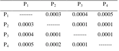
Table 4: Communication Link Failure Rate Matrix
P1 P2 P3 P4
P1 --- 0.0003 0.0004 0.0005
P2 0.0003 --- 0.0001 0.0001
P3 0.0004 0.0001 --- 0.0001
P4 0.0005 0.0002 0.0001 ---
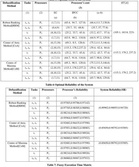
Tables-5 and 6 are showing the optimal costs and optimal reliability of the system for optimal assignment of tasks to the processors. The times have been defuzzified into crisp one by using Robust Ranking Method [RRM], Centre of Maxima Method [CoM] and Center of Area Method [CoA]. The optimal system cost on applying the Robust Ranking Method [RRM], Centre of Maxima Method [CoM] and Center of Area Method [CoA] are (105.1, 163.8, 223), (115.3, 178.2, 237.2) and (115.3, 178.2, 237.2) respectively. The optimal system reliability on applying the Robust Ranking Method [RRM],
Centre of Maxima Method [CoM] and Center of Area Method [CoA] are (0.89902,0.90055,0.94720),
(0.85650,0.90792,0.93585) and (0.85650,0.90792,0.93585) respectively.
Table 2: Fuzzy Inter Task Communication Time Matrix
t1 t2 t3 t4 t5 t6 t7
t1 (0,0,0) (4,6,8) (10,13,16) (0,2,4) (6,8,10) (1,3,5) (2,4,6)
t2 (4,6,8) (0,0,0) (15,20,24) (2,4,6) (10,12,14) (1,3,5) (10,12,16)
t3 (10,13,16) (15,20,24) (0,0,0) (3,5,7) (10,12,14) (6,8,10) (0,2,4)
t4 (0,2,4) (2,4,6) (3,5,7) (0,0,0) (6,10,16) (4,6,8) (20,25,30)
t5 (6,8,10) (10,12,14) (10,12,14) (6,10,16) (0,0,0) (0,4,6) (10,12,16)
t6 (1,3,5) (1,3,5) (6,8,10) (4,6,8) (0,4,6) (0,0,0) (2,4,6)
[image:5.595.334.525.342.425.2] [image:5.595.83.517.630.765.2]Table 5: Optimal Costs of the System Defuzzification
Method
Tasks Processors Processor’s cost
(3)
𝑅𝑇 𝐴
(1) (2) EC
(a)
IPCC (b)
(a+b)
Robust Ranking Method[RRM]
t1, t5 P1 (1,7,11) (65.4, 94.7, 127.8) (66.4,111.7,138.8)
(105.1, 163.8, 223) t2, t6 P2 (0,4,9) (35.7, 53, 68.8) (35.7, 57, 77.8)
t7 P3 (8,10,12) (25.2, 33.7, 45.4) (33.2, 43.7 , 57.4)
t3, t4 P4 (1,7,11) (63.9, 90.2, 118.8) (64.9, 97.2, 129.8)
Center of Area Method [CoA]
t1, t5 P1 (6,13,18) (69.3, 8.5, 128.6) (75.3,111.5,146.6)
(115.3, 178.2, 237.2) t2, t6 P2 (2,10,15) (115.3, 178.2,237.2) (39.4, 62.4, 84.6)
t7 P3 (8,10,12) (25.2, 33.7, 45.4) (33.2, 43.7, 57.4)
t3, t4 P4 (1,7,11) (64.7, 91.8, 118.8) (65.7, 98.8, 129.8)
Centre of Maxima Method[CoM]
t1, t2 P1 (6,13,18) (69.3, 98.5, 128.6) (75.3,111.5,146.6)
(115.3, 178.2, 237.2) t5, t6 P2 (2,10,15) (115.3, 178.2,237.2) (39.4, 62.4, 84.6)
t7 P3 (8,10,12) (25.2, 33.7, 45.4) (33.2, 43.7, 57.4)
t3, t4 P4 (1,7,11) (64.7, 91.8, 118.8) (65.7, 98.8, 129.8)
Table-6 Optimal Reliability of the System
Defuzzification Method
Tasks Processors Processor’s Reliability System Reliability(SR)
(1) (2) (3)
Robust Ranking Method[RRM]
t1, t5 P1 (0.97565,0.95786,0.97142)
(0.89902,0.90055,0.94720) t2, t6 P2 (0.97765,0.98305,0.98896)
t7 P3 (0.98216,0.98639,0.98965)
t3, t4 P4 (0.95964,0.96957,0.97893)
Center of Area Method [CoA]
t1, t5 P1 (0.92682,0.96435,0.97590)
(0.85650,0.90792,0.93585) t2, t6 P2 (0.97951,0.98432,0.98985)
t7 P3 (0.98216,0.98639,0.98926)
t3, t4 P4 (0.96060,0.96967,0.97932)
Centre of Maxima Method[CoM]
t1, t2 P1 (0.92682,0.96435,0.97590) (0.85650,0.90792,0.93585)
t5, t6 P2 (0.97951,0.98432,0.98985)
t7 P3 (0.98216,0.98639,0.98926)
t3, t4 P4 (0.96060,0.96967,0.97932)
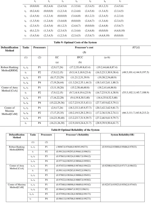
Table 7: Fuzzy Execution Time Matrix
P1 P2 P3 P4
t1 (2,6,9,12) (4,10,14,18) (4,12,15,20) (6,11,17,23)
t2 (0,3,8,12) (8,16,22,26) (7,11,15,19) (7,10,12,15)
t3 (1,5,9,14) (6,10,15,20) (6,11,14,20) (2,10,13,21)
t4 (6,13,20,27) (3,9,13,19) (0,5,7,9) (5,10,15,20)
t5 (5,7,9,11) (11,15,19,24 (8,12,16,20) (10,13,16,19)
t6 (2,9,15,20) (4,8,12,16) (6,12,18,24) (5,9,13,17)
Table 8: Fuzzy Inter Task Communication Time Matrix
t1 t2 t3 t4 t5 t6 t7
t1 (0,0,0,0) (0,2,4,6) (2,4,5,6) (1,3,5,6) (2,3,4,5) (0,1,2,3) (3,4,5,6)
t2 (0,2,4,6) (0,0,0,0) (1,2,3,4) (1,2,4,6) (2,4,5,6) (1,3,4,5) (2,3,4,5)
t3 (2,4,5,6) (1,2,3,4) (0,0,0,0) (3,4,6,8) (0,1,2,3) (2,3,4,5) (1,2,3,4)
t4 (1,3,5,6) (1,2,4,6) (3,4,6,8) (0,0,0,0) (2,4,6,7) (1,3,4,6) (2,3,4,5)
t5 (2,3,4,5) (2,4,5,6) (0,1,2,3) (2,4,6,7) (0,0,0,0) (2,4,6,8) (3,5,6,7)
t6 (0,1,2,3) (1,3,4,5) (2,3,4,5) (1,3,4,6) (2,4,6,8) (0,0,0,0) (4,6,8,10)
[image:7.595.47.550.91.784.2]t7 (3,4,5,6) (2,3,4,5) (1,2,3,4) (2,3,4,5) (3,5,6,7) (4,6,8,10) (0,0,0,0)
Table 9: Optimal Costs of the System
Defuzzification Method
Tasks Processors Processor’s cost
(3)
𝑅𝑇 𝐴
(1) (2) EC
(a)
IPCC (b)
(a+b)
Robust Ranking Method[RRM]
t1, t2 P1 (2,9,17,24) (17.2,35,49.8,63.4) (19.2,44,66.8,87.4)
(48.5,101.4,144.9,197.5) t7 P2 (7,9,12,15) (9.5,14.3,18.9,23.4) (16.5,23.3,30.9,38.4)
t4, t5 P3 (8,17,23,29) (11,21.2,31,39.9) (19,38.2,54,68.9)
t3, t6 P4 (7,19,26,44) (11.3,24.2,35.1,44.3) (18.3,43.2,61.1,88.3)
Center of Area Method [CoA]
t1, t3 P1 (3,11,18,26) (15.2,30,46,60.8) (18.2,41,64,86.8)
(55.5,102.3,145.7,188.9) t7 P2 (7,9,12,15) (9.7,14.9,19.4,23.9) (16.7,23.9,31.4,38.9)
t2, t4 P3 (7,16,22,28) (9.4,19.8,30.5,40) (16.4,35.8,52.5,68)
t5, t6 P4 (15,22,29,36) (12.7,23.9,33.5,43.1) (27.7,45.9,62.5,79.1)
Centre of Maxima Method[CoM]
t1, t2 P1 (2,9,17,24) (18.3,33.3,45.9,57.7) (20.3,42.3,62.9,81.7)
(66.3,111.7,163.8,213.2) t4, t6 P2 (7,17,25,35) (10.2,19.5,29.2,39.1) (17.2,36.5,54.2,74.1)
t3, t5 P3 (14,23,30,40) (13.2,23.7,31.9,39.7) (27.2,46.9,61.9,79.7)
t7 P4 (16,21,26,30) (12.9,18.9,24.6,31.7) (28.9,39.9,50.6,61.7)
Table10 Optimal Reliability of the System
Defuzzification Method
Tasks Processors Processor’s Reliability System Reliability(SR)
(1) (2)
Robust Ranking Method[RRM]
t1, t2 P1 (.96967,0.97648,0.98393,99273) (0.91916,0.93800,0.95686,0.97833)
t7 P2 (0.99124,0.99293,0.99461,0.99631)
t4, t5 P3 (0.97863,0.98324,0.98817,0.99412)
t3, t6 P4 (0.97716,0.98393,0.98946,0.99501)
Center of Area Method [CoA]
t1, t3 P1 (0.97453,0.98098,0.98768,0.99422) (0.92580,0.94233,0.97171,0.98432)
t7 P2 (0.99114,0.99283,0.99452,0.99631)
t2, t4 P3 (0.97883,0.98364,0.98886,0.99491)
t5, t6 P4 (0.97922,0.98364,0.98807,0.99302)
Centre of Maxima Method[CoM]
t1, t2 P1 (0.97560,0.98098,0.98689,0.99342) (0.92247,0.93923,0.95562,0.97443)
t4, t6 P2 (0.98442,0.98847,0.99233,99631)
t3, t5 P3 (0.97599,0.98128,0.98580,0.99173)
Example 2: Let us consider a fuzzy DRTS consisting a set T={t1,t2,t3,……t7} of “m=6” executable tasks and a set P=
{P1, P2, P3, P4} of “n=4” processors. The failure rates of the
processors p1,p2,p3 and p4 are 0.0002, 0.0001, 0.0003, and
0.0002 respectively. The execution time of each task on processors has been taken in the form of matrix 𝐹𝐸𝑇𝑀 = 𝑒 𝑖,𝑗 of order m x n whose elements are fuzzy trapezoidal numbers as given in Table 7. Inter tasks communication time between the tasks has been taken in the form of matrix
𝐹𝐼𝑇𝐶𝑇𝑀 = 𝑐 𝑖,𝑗 of order m whose elements are also fuzzy trapezoidal numbers as given in Table 8. Here we assume that all the communication links have the same transmission rate “wkb” and the execution cost of all the processors per unit
time in DCS is unity. The distances between each pair of processors and failure rates communication links have been taken same as taken in example1 and given in Table 3 and Table 4 respectively.
Tables-9 and 10 are showing the optimal costs and optimal reliability of the system for optimal assignment of tasks to the processors. The times have been defuzzified into crisp one by using Robust Ranking Method [RRM], Centre of Maxima Method [CoM] and Center of Area Method [CoA]. The optimal system cost on applying the Robust Ranking Method
[RRM], Center of Area Method [CoA] and Centre of Maxima Method [CoM] are (48.5,101.4,144.9,197.5),
(55.5,102.3,145.7,188.9) and (66.3,111.7,163.8,213.2) respectively. The optimal system reliability on applying the Robust Ranking Method [RRM], Center of Area Method [CoA] and Centre of Maxima Method [CoM] are (0.91916,0.93800,0.95686,0.97833),(0.92580,0.94233,0.9717 1,0.98432) and (0.92247,0.93923,0.95562,0.97443) respectively.
5.
CONCLUSION
In this paper we have introduce a new fuzzy tasks allocation problem and its solution procedure. The problem has been formulated and depicted by a mathematical model. Fuzzy execution times 𝑒 𝑖,𝑗 and fuzzy inter tasks communication times 𝑐 𝑖,𝑗 has been used while developing the model which are more realistic and general in nature. Several sets of input data are used to test the effectiveness and efficiency of model. It is found that the model is suitable for arbitrary number of processors with the random program structure.
For evaluating the performance of our algorithm a large number of programs were considered. The numbers of tasks in the examples were restricted to ten. These programs were tested for the three cases. In 1, Robust ranking, in Case-2 centre of maxima method and in Case-3, centre of area method is selected for difuzzification. We present a pair-wise comparison of each case with the other cases. In these comparisons, the percentage that each difuzzification produced better, equal or worse response time of the system is counted for the 300 task programs in the experiments. Table-11 shows the comparison results of the algorithm for these three cases. The combined column represents the percentage of the tasks programs in which the algorithm gives a better, equal or worse performance than all other cases combined.
Table-11 Pair-wise comparison of the cases
Case 1 Case 2 Case 3 Combined
Case 1 Better 80% 73% 79%
Equal - 11% 7% 7.5%
Worse 9% 20% 13.5%
Case2
Better 9% 18% 13.5%
Equal 11% - 4% 7.5%
Worse 80% 78% 79%
Case 3
Better 20% 78% 49%
Equal 7% 4% - 5.5%
Worse 73% 18% 45.5%
The ranking of the cases based on the occurrences of the best results is {case-1, case-3, and case-2}. These experiment shows that the algorithm for the case-2 is the best candidate for allocating the tasks to the processors in term of response time of the system. The present model is very useful in telephone networks, cellular network, computer games, image processing, cryptography, industrial process monitoring, simulation of VLSI circuits, sonar and radar surveillance, signal processing, simulation of nuclear reactor, power plants, airplanes, banking system etc.
6.
REFERENCES
[1] Richard R.Y., Lee E.Y.S. and Tsuchiya M., “A Task Allocation Model for Distributed Computer System”, IEEE Trans. on Computer, Vol.C-31 pp.41-47, 1982. [2] Sinclayer J.B., “Optimal Assignment in Broadcast
Network” IEEE Trans. on Computer, Vol.37 (5), pp.521-351, 1988.
[3] Casavent T.L. and Kuhl, J. G., “A Taxonomy of Scheduling in General Purpose Distributed Computing System”, IEEE Transactions on Software Engineering, Vol. 14, pp. 141-154, 1988.
[4] Sagar G. and Sarje A.K., “Task Allocation Model for Distributed System”, Int. J. System Science, Vol. 22, pp. 1671-1678, 1991.
[5] Elsade A.A. and Wells B.E. “A Heuristic Model for Task Allocation in Heterogeneous Distributed Computing System”, International Journal of Computers and Their Applications, Vol.6 (1), March 1999.
[6] Yadav P.K., Singh M.P. and Sharma K., “Tasks Allocation Model for Reliability and Cost Optimization in Distributed Computing System, International Journal of Modelling, Simulation, and Scientific Computing, Vol. 2, No.2, pp.131-149, 2011.
[7] Singh M.P., Yadav P.K. and Kumar H., Agarwal B.,
“Dynamic Tasks Scheduling Model for Performance Evaluation of a Distributed Computing System through Artificial Neural Network”, Proceedings of the International Conference on Soft Computing for Problem Solving (SocProS 2011) (Advances in Intelligent and Soft Computing: Published by Springer ) Vol.130, pp. 321-331, 2012.
[8] Bokhari, S.H. “Dual Processor Scheduling with Dynamic Re-Assignment”, IEEE Trans. On Software Engineering, Vol.SE-5 pp. 341-349, 1979.
[10] Cho S.Y. and Park K.H “Dynamic Task Assignment in Heterogeneous Linear Array Networks for Metacomputing”, Proceeding of IEEE, pp. 66-71, 1994. [11] Yadav P.K., Singh M.P. and Kumar H., “Scheduling
Algorithm: Tasks Scheduling Algorithm for Multiple Processors with Dynamic Reassignment”, Journal of Computer Systems, Networks and Communications, Article ID-578180, pp.1-9, 2008.
[12] Donight S.S.and Khanmohammadi S., “A Fuzzy Reliability Model for Series-parallel System”, J. Ind. Eng. Int., Vol. 7, No.12, pp. 10-18, 2011.
[13] Kong X., Lin C., Jiang Y., Yan W. and Chu X., “ Efficient Dynamic Task Scheduling in virtualized Data Center with Fuzzy Prediction”, Journal of Network and Computer Applications , Vol.34 , No.4, pp. 1068-1077, 2011.
[14] Kang Q., He H. and Wei J ,“An Effective Iterated Greedy Algorithm for Reliability Oriented Task Allocation in Distributed Computing System”, Journal of Parallel and Distributed Computing, Vol. 73, No.8 , pp.1106-1115, August 2013.
[15] Kumar H.,. Singh M. P and Yadav P. K, “A Task Allocation Model with Fuzz Execution and Fuzzy Inter Task Communication Times in Distributed Computing System”, International Journal of Computer Applications, Vol.72, pp. 24-31, 2013.