Financial integration and volatility in a two country world

Munich Personal RePEc Archive

Financial integration and volatility in a

two-country world

Mino, Kazuo

Institute of Economic Research, Kyoto University

March 2008

Online at

https://mpra.ub.uni-muenchen.de/16953/

Financial Integration and Volatility in a

Two-Country World

∗

Kazuo Mino

Institute of Economic Research, Kyoto University

May 2009

Abstract

This paper investigates a two-country model of capital accumu-lation with country-specific production externalities. The main con-cern of our discussion is to explore the presence of equilibrium in-determinacy in an open-economy setting. In contrast to the exist-ing studies on equilibrium indeterminacy in small-open economies, the present paper demonstrates that opening up international trade and financial interactions between two counties does not necessar-ily enhance the possibility of indeterminacy of equilibrium. It is shown that the results depend heavily upon not only on the degree of external increasing returns but also on the preference structures.

Keywords: Financial integration, Two-country growth model, Equi-librium determinacy, Preference structure

JEL classification: F43, O41

∗_{I am grateful to Eric Bond, Takashi Kamihigashi, late Koji Shimomura and Stephen}

Turnovsky for their helpful comments on earlier versions of this paper.

†_{Institute of Economic Reseach, Yoshida Honmachi, Sakyo-ku, Kyoto, 606-8501 Japan,}

1

Introduction

The equilibrium business cycle theory based on indeterminacy and sunspots

has claimed that economicfluctuations caused by extrinsic uncertainty tend

to more prominent in open economies than in closed economies. For example, inspecting a small-open economy version of the two-sector model studied by Benhabib and Farmer (1996), Weder (2001) concludes that the small-open economy requires a lower degree of external increasing returns to hold inde-terminacy than the closed-economy counterpart. Similarly, Aguiar-Conraria, L. and Wen, Y. (2005), Lahiri (2001) and Meng and Velasco (2003, 2004) also demonstrate that perfect capital mobility may enhance indeterminacy

of equilibrium for small-open economies.1 _{The main reason for this results}

is that in the small-open economies the interest rate is fixed in the world

financial market, so that consumption behaves as if the utility function were linear. Since a high elasticity of intertemporal substitutability in consump-tion serves as a cause of indeterminacy, the small-open economies tend to be more volatile than the closed economies with the same technologies and preferences.

The purpose of this paper is to examine whether the volatility of open economies emphasized by the existing studies on expectations-driven busi-ness cycles will hold in the world economy model as well. Since the world economy is a closed economy with heterogeneous agents, the present paper may be considered a study on the relationship between heterogeneity and in-determinacy.2 _{The analytical framework of this paper is a two-country model}

of capital accumulation with external increasing returns. The two countries trade consumption goods. In addition, it is assumed that agents in both countries can access to the perfect international bond market. Given such a setting, we compare the indeterminacy conditions in the autarky equilibrium with those in the world economy.3

1_{Meng and Velasco (2003, 2004) study two-sector dependent economy models with}

sector-specific externalities in which investment goods are not traded. Lahiri (2001) ex-amines a two-sector endogenous growth model with capital mobility. It is to be noted that Nishimura and Shimomura (2002b) also consider equilibrium determinacy in a two-sector small-open economy without factor mobility. Their argument follows the traditional Heckscher-Ohlin modelling.

2_{In a different context, Ghiglino and Olszak-Duquenne (2005) also consider the relation}

between heterogeneity of agents and equilibrium indeterminacy in a closed economy model of economic growth with production externalities.

3_{In the open-macroecomics literature, we have not seen any study on indeterminacy in}

Our main finding is that, as opposed to the results established in the small-open economy models, the global economy does not necessarily show a higher possibility of indeterminacy. In particular, if the preference struc-tures of both countries satisfy additive separability between consumption and labor, opening up international transactions may lower the possibility of indeterminacy. Furthermore, even in the case of non-separable utilities,

we do not find unambiguous results indicating that the world economy holds

indeterminacy under weaker restrictions on technology and preferences than the closed economies.

The rest of the paper is organized as follows. Section 2 sets up the base model. Section 3 assumes specific functional forms involved in the model and explores indeterminacy conditions under alternative assumptions on the util-ity functions. Section 4 considers a modified model that can sustain

endoge-nous long-term growth. This section reconfirms the main finding obtained

by the base model. Section 5 concludes the paper.

2

The Analytical Framework

2.1

Structure of the Model

There are two countries, country 1 and 2. Each country produces a

country-specific, single good. We assume that country 1 specializes in good x and

country 2 specializes in goody.Each good can be either consumed or invested for physical capital accumulation. It is assumed that the imported goods can be consumed, but they cannot be used as investment goods. In addition, agents in each country cannot access to the direct ownership of the foreign capital stock. However, the agents in both counties may access to the perfect international bond market so that they can freely lend to or borrow from each other. Since the international bond market is assumed to be perfect, the uncovered interest parity ensures that the nominal interest rates in both

countries are equalized in each moment. 4 _{Although our assumption that}

imported goods cannot be used for investment is restrictive, it is helpful to determine real investment in each country without introducing additional assumptions such as the presence of adjustment costs of investment.

the effect offinancial integration on macroeconomic volatility, see, for example, Evans and Hanatkovska (2005).

4_{The structure of the base model is close to the two-country model examined by}

Production

The production technology of each country is described by

zi =fi ¡

ki, li,¯ki,¯li ¢

, i= 1,2, (1)

where zi, ki and li respectively denote output, capital and labor input of

country i. In addition, k¯i and ¯li express external effects associated with the

social levels of capital and labor in country i. It is assumed that function

fi_{(.) is homogenous of degree one in k}

i and li and that it increases with

¯

ki and ¯li. This means that while the private technology under given level

of external effects satisfies constant returns, the social technology exhibits increasing returns to scale with respect to the aggregate levels of capital and

labor. We assume that those external effects are country specific so that

there are no international spillovers of production technologies.

The commodity markets in both countries are competitive. Firms maxi-mize their instantaneous profits under given levels of external effects. Hence,

lettingri andwi be the real interest rate and the real wage rate in countryi,

they respectively equal the net marginal product of capital and the marginal product of labor:

ri =fki ¡

ki, li,¯ki,¯li ¢

−δi, wi =fli ¡

ki, li,¯ki,¯li ¢

; i= 1,2. (2)

where δi ∈(0,1)denotes the depreciation rate of capital.

Households

The number of households in each country is normalized to one. The ob-jective functional of the representative household in countryiis a discounted sum of utilities such that

Ui = Z ∞

0

ui_(x

i, yi, li)e−ρtdt, ρ>0; i= 1,2,

wherexiandyi denote consumption ofxandygoods. By our assumption,y1

is exported from country 2 to country 1 andx2 is exported from country 1 to

country 2. The instantaneous utility is assumed to be increasing inxiandyi,

and decreasing in laborli.The standard concavity assumption is imposed on

ui_{(.). We assume that the households in both countries may have different}

utility functions but their discount rate is the same rate of ρ.5

Theflow-budget constraint for the households in each country is given by

˙

ωi =riωi+wili−mi, i= 1,2, (3)

where ωi is the real asset holding and mi is real consumption expenditure.

For notational convenience, ωi, wi andmi are expressed in terms of the good

countryi produces. Thus if pdenote the price of goody in terms of goodx,

the consumption spending in both countries are respectively determined by

m1 =x1+py1, m2 =

x2

p +y2.

The asset consists of capital stock, ki, and the foreign bond holding, bi.

Therefore, we define

ωi =ki+bi, i= 1,2.

where b1 and b2 are evaluated in terms of x good andy good, respectively.

The household maximizesUi subject to (3)and the initial value ofωi by

controlling consumption levels and labor supply. We impose the no-Ponzi-game condition, and hence the following intertemporal budget constraint holds as well:

ωi(0) + Z ∞

0

exp

µ

−

Z t

0

ri(s)ds ¶

wi(t)li(t)dt

=

Z ∞

0

exp

µ

−

Z t

0

ri(s)ds ¶

mi(t)dt, i= 1,2.

Market Equilibrium Conditions

Since physical capital stocks are not traded, the market equilibrium con-ditions for the commodity markets are:

z1 =x1+x2+k˙1+δ1k1, (4)

z2 =y1+y2 +k˙2+δ2k2. (5)

The world financial market is assumed to be perfect. This means that

the uncovered interest parity yields

r1 =r2+ ˙

p

p. (6)

The international borrowing and lending in the world economy should be balanced in each moment, implying that the equilibrium condition for the bond market is

b1+pb2 = 0. (7)

Note that the homogeneity of production functions gives zi = riki +wili

constraints for the home and the foreign households present the dynamic equations of b1 andb2 as follows:

˙

b1 =r1b1+x2−py1, (8)

˙

b2 =r2b2+y1 −

x2

p . (9)

Equations (8) and (9)respectively describe the current accounts of country

1 and 2.6

Perfect-Foresight Competitive Equilibrium

To sum up, the perfect-foresight competitive equilibrium (PFCE) of the

world economy is defined in the following manner:

De_finition: The PFCE of the world economy is established if the following conditions are satisfied:

(i) Thefirms maximize instantaneous profits under given levels of external effects, ¯ki. and ¯li.

(ii) The households maximize their discounted sum of utilities under given sequences of prices, {ri(t), wi(t), p(t)}∞_t=0.

(iii) Commodity markets clear and the bonds market is in equilibrium. (iv) The uncovered interest parity condition (6_{)is satisfied.}

(v) External effects satisfy consistency conditions, that is, k¯i = ki and

¯

li =li.

In what follows, we analyze the corresponding planning economy rather than the decentralized system displayed above.

2.2

A Pseudo-Planning Problem

In order to characterizes the equilibrium dynamics of the world economy, it is convenient to consider the following pseudo-planning problem:

max

Z ∞

0

£

μ₁u1(x1, y1, l1) +μ2u2(x2, y2, l2)¤e−ρtdt, μi >0, μ1+μ2 = 1

6_{We assume that the solvency conditions for international lending and borrowing are}

satisfied. Namely, the following hold:

b1(0) +

Z ∞ 0 exp µ − Z t 0

r1(s)ds

¶

x2(t)dt=

Z ∞ 0 exp µ − Z t 0

r1(s)ds

¶

p(t)y1(t)dt,

b2(0)+

Z ∞ 0 exp µ − Z t 0 ∙

r2(s) + ˙

p(s)

p(s)

¸

ds

¶

y1(t)dt=

Z ∞ 0 exp µ − Z t 0 ∙

r2(s) + ˙

p(s)

p(s)

¸

ds

¶

x2(t)

subject to

˙

k1 =f1¡k1, l1,¯k1,l¯1¢−x1−x2−δ1k1, (10)

˙ k2 =f2

¡

k2, l2,k¯2,¯l2

¢

−y1−y2−δ2k2, (11)

and given initial levels of k1(0) andk2(0). A positive constant, μi, denotes

a weight on the utility in countryi.Taking the sequences of external effects,

©_¯

k1(t),¯l1(t),k¯2(t),¯l2(t)ª∞_t=0, as given, the planner solves this problem by

selecting the optimal levels of li, xi andyi.

The Hamiltonian function for the planning problem can be set as

H = μ₁u1(x1, y1, l1) +μ2u2(x2, y2, l2)

+q1£f1¡k1, l1,k¯1,¯l1¢−x1−x2−δ1k1¤

+q2£f2¡k2, l2,k¯2,¯l2¢−y1−y2−δ2k2¤,

where qi represents the shadow value of ki. The necessary conditions for an

optimum are:

μ_iui

xi(xi, yi, li) =q1, i= 1,2, (12) μiu

i

yi(xi, yi, li) =q2, i= 1,2, (13) μiuili(xi, yi, li) =qif

i li

¡

ki, li,¯ki,¯li ¢

, i= 1,2, (14)

˙ qi =qi

£

ρ+δi−fkii

¡

ki, li,¯ki,¯li ¢¤

, i= 1,2, (15)

together with (10), (11) and the transversality conditions:

lim

t→∞e −ρt_q

iki = 0, i= 1,2. (16)

Inserting ¯ki = ki and ¯li = li into the optimal conditions, we find the

necessary conditions for an optimum of this pseudo-planning problem

com-pletely characterize PFEC conditions of the world economy defined above. .

Lemma 1 If μ₁ and μ₂ are appropriately selected, the necessary conditions for an optimum for the planning problem and the PFEC in the world economy are identical.

Proof. See Appendix 1.

2.3

Dynamical Systems

The necessary conditions for the planning problem may be summarized as a complete dynamical system with respect to the state variables, k1 andk2,

and the costate variables, q1 and q2. The structure of the dynamic system

is sensitive to the specification of the preference structure. First, consider the general case where the instantaneous utility functions are non separable ones. In this case, by use of (12) and (13), consumption demand xi and yi

may be expressed as functions of q1. q2 andki. Substituting those functions

into (14) and assuming that ¯ki = ki andl¯i = li, we find that li depends on

q1, q2 and ki. Therefore, the equilibrium levels ofxi, yi andli are written as:

xi =xi(ki, q1, q2), yi =yi(ki, q1, q2), li =li(ki, q1, q2) ; i= 1,2.

Substituting those into (10), (11) and (15) the complete dynamic system

may be written as

˙

k1 =z1(k1, q1, q2)−x1(k1, q1, q2)−x2(k2, q1, q2)−δ1k1,

˙

k2 =z2(k2, q1, q2)−y1(k1, q1, q2)−y2(k2, q1, q2)−δ2k2,

˙ qi =qi

£

ρ−ri_(k

i, q1, q2)¤, i= 1,2,

where

zi_(k

i, q1, q2) ≡ fi¡ki, li(ki, q1, q2), ki, li(ki, q1, q2)¢,

ri_(k

i, q1, q2) ≡ fk ¡

ki, li(ki, q1, q2), ki, li(ki, q1, q2)

¢

−δi.

Next, assume that the utility function is additively separable between consumption and labor in such a way that

ui_(x

i, yi, li) =φic(xi,yi) +φiL(li).

Then it is easy to see that xi and yi depend only on q1 andq2 alone, while

zι_{(.) andr}i_{(.) involve onlyk}

i and qi

˙

k1 =z1(k1, q1)−x1(q1,q2)−x2(q1,q2)−δ1k1,

˙

k2 =z2(k2, q2)−y1(q1, q2)−y2(q1, q2)−δ2k2,

˙ qi =qi

£

ρ+δi−ri(ki, qi) ¤

, . i= 1,2.

Finally, consider the case in which the utility function is additively sepa-rable for each argument, that is,

ui_(x

As demonstrated by Turnovsky (1997, Chapter 7), this assumption simplifies

the dynamic system substantially: consumption demand forxgoods depends

on q1 alone and that for y good depends on q2 alone. Thus the dynamic

system is described by

˙

k1 =z1(k1, q1)−x1(q1)−x2(q1)−δ1k1,

˙

k2 =z2(k2, q2)−y1(q2)−y2(q2)−δ2k2,

˙ qi =qi

£

ρ+δi−ri(ki, qi) ¤

, i= 1,2.

Notice that this system consists of two independent sub-system with re-spect to (k1, q1) and (k2, q2). Therefore, while the current account depends

on the foreign variables (see (8)equations(9)),consumption and investment

decisions in each country are not interdependent each other even in the fi

-nancially integrated world. Since the most general case will not produce tractable results in the base model, we focus on the second and the third cases when examining exogenous growth models in the next section. In sec-tion 4 we treats non-separable utility between consumpsec-tion and labor in the case of endogenous growth.

3

Equilibrium Dynamics

3.1

Speci

_fi

cation

In order to obtain more concrete results about determinacy of equilibrium, we now specify the production and the utility functions as the forms that have been frequently employed in the literature on indeterminacy and sunspots in the real business cycle models. The production function of each country is

zi =kα

i

i l

1−ai

i k¯ αi−ai

i ¯l βi+ai−1

, 0< ai <1, αi,βi >0, αi+βi >1.

Accordingly, imposing k¯i = ki and ¯li = li, we obtain the social production

function in each country as follows:

zi =kαiil βi

i , i= 1,2. (17)

In what follows we assume that 0 <αi <1, so that capital externalities are

not so large that unbounded growth is possible. The rate of return to capital and the real wage rate are respectively given by

ri =fki −δi =aikiαi−1l βi

i −δi, i= 1,2, (18)

wi =fli = (1−ai)kαiil βi−1

The utility function is assumed to be additively separable between con-sumption and labor. More specifically, the instantaneous utility of the house-holds in country i is given by

ui(xi, yi, li) =

⎧ ⎪ ⎪ ⎪ ⎨ ⎪ ⎪ ⎪ ⎩ ¡

xθi

i y

1−θi

i

¢1−σi

−1 1−σi −

l1+γi

i

1 +γi

, 0<θi <1, γi >0, σi >0,

θilnxi+ (1−θi) lnyi−

l1+γi

i

1 +γ_i, for σi = 1.

Given those specifications, the optimal conditions (12), (13), (14) and

(15) may be written as

μ_iθixθ

i(1−σi)−1

i y

(1−θi)(1−σi)

i =q1, i= 1,2, (20)

μ_i(1₋θi)xθii(1−σi)y

(1−θi)(1−σi)−1

i =q2, i= 1,2, (21) μil

γi

i = (1−ai)kα

i

i l βi−1

i qi, i= 1,2, (22)

˙ qi =qi

³

ρ+δi−aikαii−1l βi

i ´

, i= 1,2. (23)

3.2

Indeterminacy with Logarithmic Utility Functions

Wefirst examine the case where the utility function has a log-additive form in

consumption. Ever since Benhabib and Farmer (1994), this specification has

been most popular in the studies on indeterminacy and sunspots in the real business cycle settings. In this caseσ1 =σ2 = 1, and hence the consumption

demand functions become

xi =

1 μiθiq1

, yi =

1 μi(1−θi)q2

, i= 1,2. (24)

As pointed out in the previous section, the demand functions for each good

depend on its own price alone. On the other hand, from (21) we obtain

li =

∙ 1₋ai

μi

¸ 1

γi+1−βi

k

αi γi+1−βi

i q

1

γi+1−βi

i , i= 1,2. (25)

This states that the effects of changes in capital and commodity price on the equilibrium level of labor input depends on the sign of γi,+1−βi. If

the external effect of labor is small enough to satisfy γ_i+ 1 > β_i, then the employment level is positively related to qi and ki. If γi+ 1 <βi, the labor

In view of(10), (11), (23),(24) and(25), the complete dynamic system with logarithmic utility functions is given by the following:

˙

k1 =A1k α1(γ1+1)

γ₁₊₁−β₁

1 q

β1

γ₁₊₁−β₁

i −

∙ 1 θ1μ1

+ 1 θ2μ2

¸

1

q1 −

δ1k1, (26)

˙

k2 =A2k

α₂₍γ₂₊₁₎ γ₂₊₁−β₂

2 q

β₂ γ₂₊₁−β₂

2 −

∙ 1 (1₋θ1)μ1

+ 1 (1₋θ2)μ2

¸

1

q2 −

δ2k2, (27)

˙ q1 =q1

∙

ρ+δ1−a1A1k α₁₍γ₁₊₁₎ γ₁₊₁−β₁−1

1 q

β₁ γ₁₊₁−β₁ 1

¸

, (28)

˙ q2 =q2

∙

ρ+δ2−a2A2k α₂₍γ₂₊₁₎ γ₂₊₁−β₂−1

2 q

β₂ γ₂₊₁−β₂ 2

¸

, (29)

where

Ai =

∙ 1₋ai

μi

¸ βi γi+1−βi

, i= 1,2.

It is easy to see that the steady state equilibrium, if it exists, is uniquely determined. Letting k∗i and qi∗ be the steady-state values of capital stocks

and prices., the dynamic system linearized at the steady state is written as ⎡ ⎢ ⎢ ⎣ ˙ k1 ˙ k2 ˙ q1 ˙ q2 ⎤ ⎥ ⎥ ⎦= ⎡ ⎢ ⎢ ⎣

h11 0 h13 0

0 h22 0 h24

h31 0 h33 0

0 h42 0 h44

⎤ ⎥ ⎥ ⎦ ⎡ ⎢ ⎢ ⎣

k1−k1∗

k2−k2∗

q1−q1∗

q2−q2∗

⎤ ⎥ ⎥ ⎦,

where ∂k˙1/∂k1, h13=∂k˙1/∂q1, etc, all of which are evaluated by the

steady-state values of ki∗ and qi∗. Denote the eigenvalue of the coefficient matrix

given above by λ. Then the characteristic equation of the coefficient matrix

in the above linear system is written as

£

λ2₋(h11+h33)λ+h11h33−h13h31¤

×£λ2₋(h11+h33)λ+h22h44−h24h42¤= 0. (30)

Notice that in view of the steady-state condition, aiAik

αi(γi+1) γi+1−βi−1

i q

βi γi+1−βi

i =

ρ+δi,we obtain:

hii = A1

αi(γi+ 1)

γ_i+ 1₋β_ik

α1(γ1+1)

γ₁₊₁−β₁−1

1 q

β1

γ₁₊₁−β₁

i −δ1

= γi+ 1

γi+ 1−βi

∙

ρ+ δiβi

γi+ 1 ¸

implying that

signhii =sign (γi+ 1−βi), i= 1,2.

We also see that when γi+ 1−βi > 0, it holds that h13, h31, h24, h42 > 0

andh33, h44<0. As a result, we show that if γi+ 1−βi >0, then (30) has

two positive and two negative real roots. The presence of two-dimensional stable manifold around the steady state means that the initial levels of jump

variables, q1 and q2 can be uniquely determined. Therefore, we obtain the

following result:

Proposition 1 If the utility function is additively separable between domes-tic and imported good and production technologies of both countries satisfy γi + 1− βi > 0 (i= 1,2), then the steady state of the world economy is

determinate.

In contrast, ifγ_i+1<β_i (i= 1,2), it holds thath11, h22, h13, h24<0and

h31, h33, h42, h44, >0. Thus it is possible to have the following inequalities:

h11+h33 < 0, h11+h33<0,

h11h33−h13h31 > 0, h22h44−h24h42 >0

If this is the case, (30) have four roots with negative real parts, implying that there are a continuum of converging path near the steady state. Hence, the steady state of the world economy is at least locally indeterminate. If γ₁ + 1 > β₁ and γ₂ + 1 < β₂, then the steady state of country 2 will be

indeterminate, but that of country 1 is determinate. Since fluctuations of

country 2do not affect investment and price in country 1.

In addition, volatility in country 2 does notfluctuate the current account of country 1 either. To see this, we should note that, as shown in Appendix A, the relative price pin the market economy is proportional to the ratio of shadow values of capital,q2/q1.Given this fact, from(24)the current account

of country 1 is described by

˙

b1 = r1(k1, q1)b1+x2(q1)−

q2μ2

q1μ1

y1(q2)

= .a1A1k

α₁₍γ₁₊₁₎ γ₁₊₁−β₁−1

1 q

β₁ γ₁₊₁−β₁ 1 b1+

1 μ₂θ2q1 −

μ₂ μ2

1(1−θ1)q1

.

What is noteworthy is that the current account of country 1 depends on k1

and q1 alone. Therefore, even if the equilibrium trajectory of country 2 is

goodxis independent of the behavior ofq2.7The current account of country 1

is affected by sunspot-driven expectations only when the autarkic equilibrium of country 1 is indeterminate. In sum, we have shown:

Proposition 2 If the utility functions of both countries are logarithmic in consumption goods, then the possibility of indeterminacy will not enhanced by international trade and financial integration. Indeterminacy in one country will not spillover to the other country in any respect.

3.3

Indeterminacy with CES Utility Functions

Whenσi 6= 1 so that the utility functions are of CES forms in consumption,

equations (20) and(21) yield the following consumption demand functions:

xi =∆ixq

(1−σi)(´ 1−θi)−1

σi

1 q

−(1−σi)(σi1−θi)

2 −δ1k1, i= 1,2 (31)

yi =∆iyq

(1−σi)(1−θi)−1

σi +1

1 q

−(1−σi)(σi1−θi)−1

2 −δ2k2, i= 1,2, (32)

where

∆i x =

1 μiθi

µ

θi

1−θi

¶(1−σi)(1−θi)

>0,

∆i y =

1 μiθi

µ

θi

1₋θi

¶(1−σi)(1−θi)+1

>0.

We see that the own price effect is always negative, while the effects of foreign price on consumption demand for the home good depends on the sign of1₋σi.

If σi >1, the substitution effect dominate so that a rise in the foreign price

increases in consumption demand for the home goods. Conversely, if σi <1,

a higher foreign good price lowers demand for the home goods.

The dynamical equations in the case of non-separable utility betweenxi

andyi are thus displayed by

˙

k1 =A1k α₁₍γ₁₊₁₎ γ₁₊₁−β₁

1 q

β₁ γ₁₊₁−β₁

i −

X

i=1,2

∆i xq

(1−σi)(´ 1−θi)−1

σi

1 q

−(1−σi)(σi1−θi)

2 −δ1k1, (33)

˙

k2 =A2k

α₂₍γ₂₊₁₎ γ₂₊₁−β₂

2 q

β₂ γ₂₊₁−β₂

2 −

X

i=1,2

∆i yq

(1−σi)(1−θi)−1

σi +1

1 q

−(1−σi)(_σi1−θi)−1

2 −δ2k2, (34)

7_{If this is the case, comparative dynamics analysis by Turnovsky (1997, Chapter 7)}

together with (26) and (27).

Inspecting the dynamical system derived above, wefind that if the closed economies hold determinacy of equilibrium, opening up international trade will not enhance volatility. More formally, we obtain the following result:

Proposition 3 Suppose thatγ_i+1₋β_i >0fori= 1 and2so that the steady state in the autarkic equilibrium of both countries are locally determinate. Then the world economy holds determinacy of equilibrium for any values of σi (>0).

Proof. See Appendix B.

In this model, the price of foreign good affects capital formation of the home country only through consumption demand. The above proposition indicates that such an interaction between the two countries may not en-hance the possibility of indeterminacy. Therefore, in this case, globalization would not produce fluctuations due to extrinsic uncertainty in self-fulfilling expectations. On the contrary, globalization may be a ’stabilizing factor’, as the following proposition demonstrates:

Proposition 4 Suppose that country 1 holds indeterminacy in the autarkic equilibrium, while country 2 satisfies determinacy condition, i.e. γ₂+1 >β₂.

Then if the own price effects in the consumption demand functions dominate their cross price effect, the world economy may establish determinacy of equi-librium.

Proof. See Appendix C.

The intuition behind this result may be stated as follows. From(22) we

obtain

μ₁lγ1

1

q1

= (1₋a1)k1α1l

β1−1

1 .

Given the price, q1, and capital,k1, the left-hand side of the above expresses

labor supply curve and the right-hand side is the labor demand curve. If country 1 is a closed economy, γ1 + 1 < β1 is a necessary condition for

local indeterminacy around the steady state. As discussed by Benhabib and Farmer (1994), in this case the labor demand curve has a positive slope and it is steeper than the labor supply curve. Now suppose that country 1 is in the steady state initially. Then if the household anticipates a reduction in price, q1, the labor supply curve shifts up, implying that labor employment

and production increase. Since a lower price raises the domestic demand for

a rise in production. This means that the initial anticipation of a lower price will be self fulfilling. In the world economy, the mechanism that may generate indeterminacy is essentially the same as that in the close economy. If the households in the world anticipated a decrease in q1,the consumption

demand for x goods increase. This again makes the labor supply curve in

country 1 shifts up, which raises the production level of x. However, in

the case of world economy a lower q1 increases the export for country 2 as

well as the domestic consumption demand. If such a demand effect is large enough, a rise in employment in country 1 is insufficient to satisfy the newly created consumption demand. In this case the initial anticipation cannot be self fulfilled. Therefore, the equilibrium is determinate even though labor externalities are sufficiently large to satisfy γ₁+ 1<β₁.

4

Endogenous Growth

So far, we have considered a model of exogenous growth in which the world economy will not display sustained growth in the steady-state equilibrium. In this section, we consider an endogenously growing world economy by mod-ifying the base model. It is shown that in the case of endogenous growth we may treat a lower dimensional dynamic system than in the base model. This enables us to examine the model with nonseparable utilities between consumption and labor supply in which there is a strong interdependency between the two countries.8

In the following, we assume that both countries have Ak technologies

in the sense that their production functions are linearly homogenous with respect to the private and the social levels of capital. Hence, we assume that α1 = α2 = 1, implying that the social production function in each country

becomes

zi =ka

i

i l

1−ai

i k¯

1−αi

i ¯l βi+ai−1

i =l

βi

i ki, i= 1,2. (35)

As a result, the rate of returns to capital are given by

ri =ail βi

i −δi, i= 1,2. (36)

4.1

Separable Utility

Wefirst inspect the model with spareable utility functions. As is well known, if the utility function is additively separable between consumption and labor,

8_{The model in this section is an example of two-country model of endogenous growth.}

the sub-utility generating from consumption should be logarithmic to hold balanced growth equilibrium with a positive growth rate. Thus in this section we assume that σi = 1, so that

ui_(x

i, yi, li) =θilnxi + (1−θi) lnyi−

l1+γi

i

1 +γi

.

Given this function, (14) yields

lγi+1−βi

i = (1−ai)qiki, i= 1,2.

Let us denoteqiki =vi. Then the equilibrium level of employment in country

i is

li =ηiv 1

γi+1−βi

i , i= 1,2. (37)

whereη_i = (1₋ai) 1

γi+1−βi _{.The equilibrium employment level in each country}

increases (resp. decreases) with the value of capital, if γi + 1 > βi.(resp.

γ_i+ 1 <β_i). In this case, the demand functions forfinal goods are given by

xi =μiθi/qi, yi =μi(1−θi)/qi, i= 1,2. (38)

By use of (24), we show that the growth rates of capital stocks in both

countries are expressed as follows:

˙ k1

k1

=η₁v

β₁ γ₁₊₁−β₁

1 −

μ₁θ1+μ2θ2

v1 −

δ1,

˙ k2

k2

=η₂v

β2

γ2+1−β2

2 −

μ1(1−θ1) +μ2(1−θ2)

v2 −

δ2.

The price in each good changes according to

˙ qi

qi

=ρ₋ailβii, i= 1,2.

By the definition of vi(=qiki), we thus obtain:

˙ v1

v1

= (1₋a1)η1v β₁ γ₁₊₁−β₁

1 +ρ−

μ₁θ1+μ2θ2

v1 −

δ1, (39)

˙ v2

v2

= (1₋a2)η2v β₂ γ₂₊₁−β₂

2 +ρ−

[μ₁(1₋θ1) +μ2(1−θ2)]

v2 −

δ2. (40)

Differential equations (39) and (40) constitute a complete set of dynamic

The balanced-growth of the world economy is attained when v˙1 = v˙2 =

0. Note that in the balanced growth equilibrium, the real income of both

countries need not grow at a common rate. If each country grows at a different rate, the relative price betweenxandygoods continue to change at a constant rate to keep the uncovered interest parity condition,r1 =p/p˙ +r2.

Hence, letting gi be the steady-growth rate of country i, in the

balanced-growth equilibrium, we obtain

gi =ailβii−ρ−δi =−q˙i/qi, i= 1,2, (41)

which means that change in the relative price on the balanced-growth path is

˙ p p =

˙ q1

q1 −

˙ q2

q2

=a2l2β2 −a1l1β1 +δ1−δ2. (42)

The rate of change in asset holding in country 1 is given by

˙ b1

b1

=g1+ρ+ μ₁θ1

q1b1 −

pμ₂(1₋θ2)

q2b1

.

In the balanced-growth equilibrium b1 changes at the rate of g1 and thus it

holds that

pμ₂(1₋θ2)

q2b1 − μ₁θ1

q1b1

= py1 −x1

b1

=ρ.

Similarly, the balanced-growth condition in country 2 involves x2/p −y1 = ρb2.

Due to the assumption of log-additive utility functions, there is no inter-action between the dynamic behaviors of v1 and v2. It is easy to confirm

that the steady-state value of vi is uniquely given if γi + 1 > βi. We also

find that if γi + 1 < βi, then either there is no steady state or there are

dual steady states. Here we assume that both countries have dual balanced-growth paths whenγ_i+1<β_i.Additionally, we can confirm that when there are two steady state, one with a lower value ofviis locally indeterminate and

the other with a higher value of vi is locally determinate.9 Consequently, we

may state:

Proposition 5 Ifγi+1−βi >0fori= 1,2,the world economy has a unique

balanced growth path that satisfies global determinacy. On the contrary, if γ_i + 1₋β_i <0 for i = 1,2, then there may exist four steady states: one in which both country grow at the lower rate is locally determinate, while the other three are locally indeterminate.

9_{Denote the steady state values of vi as v}∗

i and vi∗∗ (vi∗ < vi∗∗). It is seen that that

dv˙i/dvi < 0for vi = v∗i and dv˙i/dvi > 0 for vi = vi∗∗. Since vi is not a predetermined

Figure 1-a depicts the phase diagram of (39) and (40) for γi + 1 > βi

(i= 1,2) (so that the world economy is globally determinate). If this is the case, the world economy stays on the balanced-growth path and it has no transitional dynamics. In contrast, if γi + 1 <βi (i = 1,2), then the world

economy involves four steady states: the balanced-growth path on which both countries attain lower growth rates will not display indeterminacy, while other three are locally indeterminate. As Figure 1-b shows, the steady state where both countries attain higher growth rates is a sink. This suggests that the behaviors of the terms of trade and current accounts of both countries may be totally indeterminate around on the high-growth steady state of the world economy.

It is worth emphasizing that in our setting each country may attain a different rate of balanced growth. In particular, in the case of Figure 1-b, the balanced-growth rate of each country may differ from each other even though both countries have the identical production and preference structures. This is because the balanced growth path where country 1 (country 2) grows faster than country 2 (country 1) may be attained as a steady state equilibriums the world economy even in the presence of free trade and a well-organized international financial market.

4.2

Non-Separable Utility

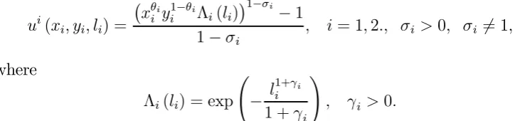
We now assume that the utility functions are non-separable between con-sumption and labor. We specify the instantaneous utility function is given by

ui(xi, yi, li) = ¡

xθi

i y

1−θi

i Λi(li) ¢1−σi

−1 1−σi

, i= 1,2., σi >0, σi 6= 1,

where

Λi(li) = exp Ã

− l

1+γi

i

1 +γi !

, γ_i >0.

Whenσi = 1,the utility function takes a log-additive form used before. The

necessary conditions for an optimum for the planning problem involve the following conditions:

μ_iθix(1−σ

i)θi−1

i y

(1−σi)(1−θi)

i Λi(l)

1−σi

=q1, (43)

μ_i(1₋θi)xθii(1−σi)y

(1−θi)(1−σi)−1

i Λi(li)1−σ

i

=q2, (44)

μ_ix(1−σi)θi

i y

(1−σi)(1−θi)

i Λ0i(li)Λi(li)−σ

i

˙ qi =qi

h

ρ+δi −ailβii i

. (46)

From(43), (44) and (45), the consumption demand functions are given

by

x1 =θ1(1−a1)l1β1−γ1−1k1

x2 =

q2

q1

θ2(1−a2)l2β2−γ2−1k2

y1 =

q1

q2

(1₋θ1) (1−a1)l1β1−γ1−1k1

y2 = (1−θ2) (1−a2)lβ22−γ2−1k2

Given the non-separable utilities, consumption demand in each country is directly related to capital and labor input as well as to the relative price.

Observe that substituting those demand functions into (43) and(44) yields

Φ1k1−σ1q

(1−σ1)(1−θ1)

1 q−

(1−σ1)(1−θ1)

2 l

σ1(1+γ₁−β₁)

1 exp

µ

−(1₋σ1)

lγ1+1

γ₁+ 1

¶

=q1,

(47)

Φ2k−2σ2q−

(1−σ2)θ2

1 q

(1−σ2)θ2

2 l

σ2(1+γ2−β2)

2 exp

µ

−(1₋σ2)

lγ2+1

γ2+ 1

¶

=q2, (48)

where Φ1 and Φ2 are positive constants. Those equations show that the

equilibrium level of l1 depends onk1, q1 and q2, while that ofl2 depends on

k2, q1 andq2.

Logarithmic differentiation of both sides of (47) and (48) with respective to time yields the following relations:

˙ l1

l1

= 1

σ1(1 +γ1−β1)−(1−σ1)lγ11+1

"

σ1

˙ k1

k1

+ [1₋(1₋σ1) (1−θ1)] ˙

q1

q1

+ (1₋σ1) (1−θ1) ˙

q2 q2 ¸ , ˙ l2 l2

= l2

σ2(1 +γ2−β2)−(1−σ2)lγ22+1

"

σ2

˙ k2

k2

+ (1−σ2)θ2 ˙

q1

q1

+ (1₋θ2+σ2θ2) ˙

q2

q2

¸

.

On the other hand, from (10) and (11) we obtain:

˙ k1

k1

=lβ1

1 −θ1(1−a1)l1β1−γ1−1−mθ2(1−a2)l2β2−γ2−1−δ1 ≡κ1(l1, l2, m)

˙ k2

k2

=lβ2

2 −(1−θ1) (1−a1)

lβ1−γ1−1

1

m −(1−θ2) (1−a2)l

β2−γ2−1

2 −δ2 ≡κ2(l1, l2, m),

(50) where m = q2k2/q1k1. Using those relations, we obtain the following

differ-ential equations:.

˙ l1 =

l1

∆1(l1)

h

σ1κ1(l1, l2, m) + [1−(1−σ1) (1−θ1)]

³

ρ−a1lβ11

´

+ (1₋σ1) (1−θ1)

³

ρ₋a2lβ22

´i

, (51)

˙ l2 =

l2

∆2(l2)

h

σ2κ2(l1, l2, m) + (1−σ2)θ2

³

ρ₋a1l1β1

´

+ (1−θ2+θ2σ2)

³

ρ−a2l2β2

´i

, (52)

˙

m=mhκ2(l1, l2, m)−κ1(l1, l2, m) +a1l1β1 −a2l2β2

i

, (53)

where

∆i(li) =σi(1 +γi−βi)−(1−σi)l γi+1

i , i= 1,2.

Dynamic equations (51), (52) and (53) present a complete system of l1, l2

andm (=q2k2/q1k1).

The balanced-growth equilibrium is attained whenli andmstay constant

over time, which means that the growth rate of income in each country is constant and the relative price satisfies (.42). We assume that the dynamic

system involves a feasible stationary solution. As shown by (47) and (48),

once the initial values ofkiandqiare selected, the initial values ofl1andl2are

determined as well. This indicates that under a given level of k2(0)/k1(0),

the initial levels of l1,l2 andm cannot be chosen independently: only two of

them are unpredetermined. Therefore, if the linearized system of (51), (52) and(53)involves one stable and two unstable roots, then the balanced-growth equilibrium is locally determinate. If the approximated system has at least two stable roots, then the balanced-growth path is locally indeterminate.

When the utility function is not additively separable between

consump-tion and labor, dynamic behavior of the closed-economy of country i is

ob-tained by setting θ1 = 1 andθ2 = 0, respectively. Thus the dynamic system

of closed economy is

˙ li =

li

σi(1 +γi−βi)−(1−σi)lγii+1 h

(σi−ai)liβi +ρ−(1−ai)liβi−γi−1 i

.

We now find that either if

or if

γ_i+ 1<β_i andσi < ai, i= 1,2, (55)

then each country has a unique balanced-growth path that satisfies global

determinacy. Inspection of the world economy dynamics given by(51), (52)

and (53) shows that if (54) holds, it is hard to establish indeterminacy in

the world economy. However, if conditions in (55).are fulfilled, the world

economy tends to have indeterminate equilibria.

Proposition 6 If γi + 1 > βi and σi > ai then both the closed and the

world economies may hold determinacy of equilibrium. If γi + 1 < βi and

σi < ai, then the world economy has indeterminate equilibria, while each

closed economy does never have indeterminacy.

Proof. See Appendix D.

Although the non-separable preferences increase interdependency between two counties, the above proposition suggests that such a stronger relationship does not necessarily produce complex dynamics. This result is an example showing that internationalization of markets under complex preference struc-tures may or may enhance the possibility of multiple equilibria and sunspots

fluctuations. Unlike small-open economies where openness usually presents

a higher possibility of indeterminacy, such an unambiguous relationship may not exist in the global economic system.

5

Conclusion

The central message of this paper is that the relation between indeterminacy of equilibrium and openness of the economy is sensitive not only to produc-tion technologies but also to preference structure. By use of a two-country models withfinancial integration, we have examined whether or notfinancial interactions and international trade enhance the possibility of indeterminacy. We have found that, as opposed to the results shown by the existing stud-ies on small-open economstud-ies, opening up international transactions does not necessarily yield a higher possibility of indeterminacy. On the contrary, in some cases globalization may serve as a ’stabilizing factor’ in the sense that the equilibrium path of the world economy can be determinate even though

the autarky equilibrium of each country is indeterminate. Since our finding

depends heavily upon the model structure we use in the paper, it may not be appropriate to claim that the global economy is in general less volatile than closed economies. However, our analysis has suggested that the

Appendices

Appendix A: Proof of Lemma 1

First consider the optimization behavior of the households in country i. The Hamiltonian function for the household’s problem is

Hi =ui(xi, yi, li) +vi(riΩi+wili−mi), i= 1,2,

where m1 =x1 +py1 and m2 = x2/p+y2. The necessary conditions for the

optimization problems are summarized as follows:

u1

x(x1, y1, l1) =v1, ux2(x2, y2, l2) =v2/p, (A1)

u1_y(x1, y1, l1) =pv1, u2y(x2, y2, l2) =v2, (A2)

ui

l(xi, yi, li) =viwi, i= 1,2, (A3)

˙

vi/vi =ρ−ri, i= 1,2, (A4)

lim

t→∞vie −ρt_ω

i = 0, i= 1,2. (A5)

Keeping the non-arbitrage condition (6) in mind, the equations in (??)

present

˙ p

p =r1−r2 = ˙ v2

v2 −

˙ v1

v1

.

This shows that the relation between the relative price, p,and the marginal utility of capital, vi, must satisfy

p=μv2

v1

, (A6)

where μis a positive constant. From(??) μsatisfies

μ= u

2

x(x2, y2, l2)

u1

x(x1, y1, l1)

.

Thus if the economy involves a steady state in which each variable stays constant over time, substituting the steady-state values of xi, yi and li into

the above equation determines the magnitude of μ.

From (A1), (A2) and (A6) we obtain

u1

y

u1

x

= u

2

y

uyx

=p=μv2

v1

, u

2

x

u1

x

= u

2

y

u1

y

= v2

v1p

Now remember that the optimal conditions (12) and (13) for the planning problem yield: u1 y u1 y

= q1

q2 = u 2 y u2 x , u 2 x u1 y = u 2 y u2 y

= μ1

μ₂. (A8)

Therefore, if we set q1/q2 = p and μ1/μ2 = μ, (A7) and (A8) receptively

correspond to (12) and (13) for the planning problem, so that the optimal conditions for the consumption decisions in the market economy and those in the planning economy are exactly the same. In addition, the optimal conditions for labor supply (A3) is identical to (14) in the planning problem and the commodity market equilibrium conditions (4) and (5) are described by (10) and (11), repetitively.

Finally, the solvency conditions for international lending and borrowing requires that

lim

t→∞b1(t) exp

µ

−

Z t

0

r1(t)ds

¶

= lim

t→∞b2(t) exp

µ

−

Z t

0

r2(s)ds

¶

= 0.

Thus the transversality conditions (A5) givelimt→∞e−ρtvitkit= 0 (i= 1,2).

Since we may set qi =μivi,conditions in (A5) are equivalent to (16) for the

planning problem.

Appendix B: Proof of Proposition 3

The dynamic behavior of the closed economy is described by

˙ ki =k

αi(γi+1) γi+1−βi

i q

βi γi+1−βi

i −

1

qi −

δi, (B1)

˙ qi =qi

"

ρ+δi−aik

αi(γi+1) γi+1−βi−1

i q

βi γi+1−βi

i

#

. (B2)

Linearizing (B1) and (B2) at the steady-state equilibrium, it is easy to see that the trace of the coefficient matrix equals toρ(>0).On the other hand, the coefficient matrix of the linearized system of (33), (34), (26) and(27)is given by:

Λ(λ) =

¯ ¯ ¯ ¯ ¯ ¯ ¯ ¯

λ−h11 0 −h13 −h14

0 λ−h22 −h23 −h24

−h31 0 λ−h33 0

0 −h42 0 λ−h44

¯ ¯ ¯ ¯ ¯ ¯ ¯ ¯

= 0,

the steady state. The characteristic equation is thus written as

Λ(λ) =£λ2−(h11+h33)λ+h11h33−h13h31

¤

×£λ2−(h22+h44)λ+h22h44−h24h42

¤

−h14h23h31h42= 0. (B3)

Given our assumptions, ifh14 =h23 = 0, then Λ(λ) = 0 has two positive

and two negative roots. Thus if the number of negative roots of Λ(λ) = 0 is higher than three forh14 6= 0 andh23 6= 0,then the steady state of the world

economy is locally indeterminate. Notice that

Λ(0) = (h11h33−h13h31) (h22h44−h24h42)−h14h23h31h42,

Λ0_{(0) =−(h}

11+h33) (h22h44−h24h42)−(h22+h44) (h11h33−h13h31).

As well as the closed system, ifγi+ 1>βi (i= 1,2)holds,h11+h33>0and

h22+h44 >0.In addition, the saddle-point properties of the closed economies

mean that h22h44−h24h42 < 0 and h11h33−h13h31 < 0. Hence, Λ0(0) > 0

andΛ(0) >0for h14=h23= 0.This shows that Λ0(λ) = 0 has two positive

and one negative roots, and thus when h14 = h23 = 0, the graph of the

characteristic equation may be depicted as Figure A1. Therefore, regardless of the sign of h14h23h31h42, the characteristic equation, Λ(λ) = 0, has at

most two negative roots.

Appendix C: Proof of Proposition 4

Since country 1 has an indeterminate steady state and country 2 has a determinate one, (B3) involves three negative and one positive roots when

h14 = h23 = 0. Namely, Λ(0) in Appendix B has a negative value if h14 =

h23 = 0. Observe thatΛ(0) can be written as

Λ(0) = h11h22h33h44−h11h42h24h33−h31h13h22h44

+h31h42(h13h24−h14h23).

Under our assumption,γ1+1<β1 andγ2+1 >β2,it holds thath31>0and

h42 >0. Therefore, if

h13h24−h14h23<0, . (C1)

then Λ(0) may have a positive sign. As Figure A2 shows, if this is the case, the characteristic equation has two positive and two negative roots so that

the steady state of the world economy is determinate. Condition (C1) is

equivalent to

à X

i=1,2 ∂xi

∂q1

! Ã X

i=1,2 ∂yi

∂q2

!

−

à X

i=1,2 ∂xi

∂q2

! Ã X

i=1,2 ∂yi

∂q1

!

which states that the own price effects on consumption demand dominates the cross price effects.

Appendix D: Proof of Proposition 6

Ifγ_i+ 1>β_i andσi >1,then∆i(li) = (γi+ 1−βi)−(1−σi)liγi+1 >0.

Assume that the dynamic system has a feasible steady-state equilibrium. Linealized system has the coefficient matrix such that

J = ⎡

⎣ l1/0∆1 l2/0∆2 00

0 0 m

⎤ ⎦

⎡ ⎣

J11 J12 σ1κ1m

J21 J22 σ2κ2m

κ2

1−κ11−a1β1l

β1

1 κ22 −κ12+a2β2l

β2−1

2 κ2m−κ1m

⎤ ⎦,

(C1) where

κ1(l1, l2, m) =l1β1 −θ1(1−a1)l1β1−γ1−1−mθ2(1−a2)l2β2−γ2−1,

κ2(l1, l2, m) =l2β2 −(1−θ1) (1−a1)

lβ1−γ1−1

1

m −(1−θ2) (1−a2)l

β₂−γ₂−1

2 ,

and κj_i = ∂κj_/∂q

i > 0 (i, j = 1,2), κ1m = ∂κ1/∂m < 0, κ2m = ∂κ2/∂m >

0.and

J11 = σ1κ11−a1β1[1−(1−σ1) (1−θ1)]l1β1−1,

J12 = σ1κ12−a2β2(1−σ1) (1−θ1)lβ22−1 >0,

J21 = σ2κ21−a1β1(1−σ2)θ2lβ11−1 >0,

J22 = σ2κ22−a1β2(1−θ2+θ2σ2)l2β2−1.

From the determinacy condition for the closed economy, it may hold that

J11>0 andJ22>0. In view of those sign patterns, we find that

detJ <0and trace J >0.

This confirms that the dynamic system involves one stable and two unstable

roots. Hence, the world economy also satisfies determinacy.

Ifγi+ 1<βi andσi < ai,then J11>0andJ22 >0still may hold. Since κi

j (i6=j) < 0, we obtain J12 < 0 and J21 < 0. Remembering that in this

case ∆i_(l

i)<0,we see that

detJ >0and trace J <0.

References

[1] Aguiar-Conraria, L. and Wen, Y. (2005), "Foreign Trade and Equilib-rium Indeterminacy", Working Paper 2005-041A, Federal Reserve Bank of St. Louis.

[2] Baxter, M. and Crucini, M.J. (1995), ”Business Cycles and the Asset

Structure of Foreign Trade”, International Economic Review 36,

821-854.

[3] Benhabib, J. and Farmer, R.E.A. (1994), ”Growth and Indeterminacy”, Journal of Economic Theory 63, 19-41.

[4] Benhabib, J. and Farmer, R.E.A. (1996), "Indeterminacy and Sector-Specific Externalities",Journal of Monetary Economics

[5] Evans, D. M. and Hnatkovska, V. (2006), "Financial Integration, Macro-economic Volatility and Welfare", unpublished manuscript.

[6] Ghiglino, C. and Olszak-Duquenne, M. (2005), "On the Impact of Het-erogeneity on Indeterminacy", International Economic Review 46, 171-188.

[7] Farmer, R.E.A. and Lahiri, A. (2005), "A Two-Country Model of

En-dogenous Growth," Review of Economic Dynamics 8, 68-88.

[8] Farmer, R.E.A. and Lahiri, A. (2006), “Economic Growth in an

Inter-dependent World Economy”, Economic Journal 116, 969-990.

[9] Lahiri, A. (2001), ”Growth and Equilibrium Indeterminacy: The Role

of Capital Mobility”, Economic Theory 17, 197-208.

[10] Meng, Q. and Velasco, A (2003), "Indeterminacy in a Small Open

Econ-omy with Endogenous Labor Supply," Economic Theory 22, 661-670.

[11] Meng, Q. and Velasco, A (2004), "Market Imperfections and the In-stability of Open Economies," Journal of International Economics 64, 503-519.

[12] Mino, K. (2001a), ”Indeterminacy in Two-Sector Endogenous Growth Models with Leisure”, unpublished manuscript.

[13] Mino, K. (2001b), ”Indeterminacy and Endogenous Growth with Social

[14] Nishimura, K. and Shimomura, K. (2002a), ”Indeterminacy in a

Dy-namic Small Open Economy”,Journal of Economic Dynamics and

Con-trol 27, 271-281.

[15] Nishimura, K. and Shimomura, K. (2002b), "Trade and Indeterminacy in a Dynamic General Equilibrium Model",Journal of Economic Theory 105, 249-259.

[16] Nishimura, K. and Shimomura, K. (2006), ”Indeterminacy in a Dynamic

Two-Country Model", Economic Theory 29, 307-324.

[17] Obstfeld, M. and Rogoff, K. (1996),Foundations of International

Macro-economics, MIT Press, Cambridge, MA.

[18] Pelloni, A. and Waldmann, R.(1998), ”Stability Properties of a Growth

Model”, Economics Letters 61, 55-60.

[19] Weder, M. (2001), ”Indeterminacy in a Small Open Economy Ramsey

Model”, Journal of Economic Theory 98, 339-356.

[20] Wen, Y. (2001), ”Understanding Self-Fulfilling Rational Expectations

Equilibria in Real Business Cycle Models”, Journal of Economic

Dy-namics and Control 25, 1221-1240

[21] Turnovsky, S. (1997), International Macroeconomic Dynamics, MIT

Press, Cambridge, MA.