Munich Personal RePEc Archive
Who does the chores? Estimation of a
household production function in Peru
Garcia, Luis
Departamento de Economia, Pontificia Universidad Catolica del
Peru
2007
Online at
https://mpra.ub.uni-muenchen.de/23223/
Who does the chores? Estimation of a household production
function in Peru
+Luis Garcia
a,*a Department of Economics, Pontifical Catholic University of Peru, Av. Universitaria 1801, San Miguel, Lima 32, Peru
June 2007
Abstract
In less developed countries like Peru, it is very frequent to observe that, in poor households, parents and children work together doing household work in their own home. This fact is even more evident among girls, who work at home cleaning, cooking, taking care of younger siblings, etc., which may deter them from attending school. In the current literature on child labour, it is always assumed that this occurs because girls are more productive at home than boys; therefore is more likely to observe girls staying home and boys working in the labour market. To check to what extent this common assumption is true, this paper estimates the determinants of household work in Peru, and obtains the parameters of the production function of “chores”. Since the total amount of “chores” is not observable, I use wages and the first order conditions of a standard time allocation model to estimate the model. The estimated production function is consistent with a strictly concave production function in which the inputs are substitutes. It also shows that girls have a higher marginal product than boys in the production of “chores”. All data was taken from the Peruvian Living Standard Measurement Survey of 1997 and 2000.
________________________
JEL classification: D13, J22. Keywords: time allocation, household work, child labor.
* Corresponding author: Phone: (511)626-2000 Ext.4976, Fax: (511) 626-2874, email address: [email protected].
+
Who does the chores? Estimation of a household production function in Peru
1. Introduction
In recent years, literature on child labour has paid special attention to the work of children as household workers, work which is understood as that performed at home involving the production of output for direct family consumption, but not for market sale.1 Like standard child labour, household work consumes time and effort, which leaves less time for children to do other
activities, like studying. It could also deter girls in less-developed countries from attending school, as some papers suggest.2
To give an idea of the magnitude of this phenomenon, in Peru (a poor and less-developed country), three of every four children work some positive number of hours per week on housework, where the total average of hours worked is roughly 11 hours per week. In the six-to-fourteen-year age range, poor girls work at home, on average, twice as much as non-poor boys do. In addition, girls who do not attend school work more hours on housework than girls who do attend school, and the gap between those averages increases with age.3
These facts suggest that it is important to study and understand this phenomenon from an economic point of view. What makes adults and children work in this activity? What variables could increase or decrease the time individuals spend on housework? Why is it that we observe more housework performed by girls than by boys? Literature on household economics offers models that can be used to examine this problem in depth. To answer these questions, I find the main determinants of household work and estimate a household production function, controlling by those variables that affect the production function. Using econometric methods and survey data, this paper achieves both tasks.
In the setting proposed in this paper, wages play an important role in the time allotted to household work, since wages are the opportunity costs of hours spent on this activity. Standard neoclassical
1
Household work includes activities like cleaning, cooking, taking care of younger children, etc.
2
Levison and Moe (1998).
3
theory predicts a negative relationship between wages and hours of housework. In addition – as will be clear in the empirical section — wages are an important instrument in the estimation of the parameters of the production function.
It is also important to note that household work is not always seen as a “bad thing” for children, because it can create a sense of responsibility in children and develops skills that will be useful in the future. It is reasonable to think about an “acceptable” level of household work performed by children. The problem with household work occurs when parents make children work so many hours that they do not have enough time to study, play or rest. Parents can use household work as a strategy to increase a family’s total income, in the sense that if children do the chores at home, the parents may have more free time to offer in the labour market.4
Besides classical papers on the theory of allocation of time (Becker, 1965; Gronau, 1977; Rosenzweig, 1980; Birdsall, 1982; Newman & Gertler, 1994), some works have developed this theory in the context of household work with child workers. For example, Brown et al. (2003) present a theoretical model of child labour with household work, but assume a Ricardian
production function with fixed coefficients, which yields specialisation of children in housework or market work. Recently, Garcia (2006) has presented a theoretical model which approaches this problem using the “unitary approach”5, in which household work, child labour, and hours of children’s education are determined simultaneously along with the parents’ labour supply and household work. In that model, we do not observe specialisation; the time is allocated according to the opportunity cost of the activities individuals may perform.
Several empirical papers estimate the determinants of child labour, schooling, and household work under the time-allocation framework and using Probit or Tobit methods, while others use
simultaneous-equations methods. Skoufias (1994) studies the effect of market wages on time allocation in rural India. This study shows significant differences between boys and girls when it comes to participation in productive activities within the household and schooling. Using average
4
Skoufias (1994) proposed this idea.
5
community wages to estimate parents’ and children’s wages, the author finds that wages have no effect on participation in household production activities, and that only the child’s wage has a negative effect on leisure and a positive effect on the remaining activities – home production, schooling and market work. DeGraff et al. (1996), using data from the Philippines, estimate a simultaneous Probit model in which the endogenous variables are dummy variables of school attendance, market work and household work. They find that household work increases with age, and that its incidence is higher for girls. Some household characteristics such as number of siblings and housing material have an impact on the hours worked by children at home. In a later paper, DeGraff and Bilsborrow (2003) estimate the same model using the same exogenous variables, but this time they estimate only the reduced form equations by the Tobit method; however, their results are not good because almost none of the variables are a good predictor of household work hours. Levison & Moe (1998) analyse household work as a deterrent to schooling. Focusing on unmarried adolescent girls ages 10 to 19, they find that household work may present a more significant barrier to schooling for girls than boys. They do not include wages in the regressions. Binder and Scrogin (1999) estimate the determinants of child work in Mexico. In particular, they focus their attention on the effect of parents’ wages and children’s wages on their labour decisions. Using imputed child wages, they find a negative effect on the participation of children in
substantial household responsibilities. They also find that this participation is lower for boys and for younger siblings. Hours worked in housework are also fewer for boys than for girls.
In short, the current literature on this topic has identified some of the main variables that determine housework. However, it has not considered the interaction between parents’ and children’s
housework in the production of chores nor has it estimated this production function. In addition, most papers report that girls work more hours than boys at home, and provide explanations for this result related to customs and differences in productivity. Here I do not assume that girls are more productive at home than boys, but the estimation results show that indeed girls are more productive at home.
The paper is organised as follows: section 2 summarises the empirical model to be estimated and describes the econometric strategy to conduct the estimations; section 3 briefly describes the data; section 4 presents and discusses the results, and finally, section 5 concludes.
2. The Empirical Model
In this section, I briefly review the model presented in Garcia (2006) and derive the econometric specification. The model is a standard model of time allocation where household work has been included as a single activity that the children and one of the parents can perform. The time spent on this activity produces a certain level of output which represents total amount of housework done (for example, how clean or neat the house is). To simplify the model, it is assumed that there are only three individuals in the household: the head of household, the spouse and only one child. 6 The spouse spends her time (T) in household work (z1) or market work (H1) thus her time
constraint is z1H1 T, but the head of household only works full time in the labour market. The child may spend her time studying (E), working at home doing housework (z2) or working in the labour market (H2), thus her time constraint is z2H2ET. The head of household is the family planner who allocates the time of the spouse and the child to maximise the aggregated family utilityU(c,Z,E) where c is the total aggregated consumption, Z the total level of housework produced. Housework can be produced at home or bought in the market, so its total amount is expressed by the equation Z f0 f(z1,z2), where f0 are the hired domestic services, and f(z1,z2) is a strictly concave home production function whose inputs are the hours that the
6
spouse and the child spend at home doing housework. The household faces a budget constraint, where the aggregated household income is the sum of the labour income of the head of household (Y), the spouse (w1H1) and the child (w2H2), and the total expenditure is cPf0, where c represents the family consumption of a composite good (whose price is set to one) and P is the price of housekeeping service. The optimisation problem the family planner solves is to maximise the utility function subject to the time constraints, the budget constraint and the equation which defines the total amount of Z.7
The strategy to estimate the structural parameters of the model is to obtain information from the first order conditions. According to the solution of the theoretical model and assuming the interior solution, the first order conditions yield:
P w z z
f1( 1, 2) 1 (1)
P w z z f 2 2 1
2( , ) (2)
where fi is the marginal product with respect to input i. Equations (1) and (2) determine the optimal values of the household work variables z1z1(w1,w2,P) and z2 z2(w1,w2,P) which are the demands for child and spouse’s household work.
The total output of chores is not observed; we only observe the time employed in that activity. However, by working with the first order conditions we can recover the structural parameters of the production function.
The first order conditions (1) and (2) say also that the marginal product of inputs must equal the ratio of wages with respect to the price of housekeeping services (the opportunity cost of
household work). It is also true that
2 1 2 1 2 2 1 1 ) , ( ) , ( w w z z f z z f (3) 7
so the family will allocate the time such that the ratio of marginal products equals the ratio of wages.
The next step is to define a parametric functional form for the production function. In the
theoretical model we assumed the home production function is a concave function. For empirical purposes it is convenient to assume a quadratic function8
z z z
b z
f
2 1 )
( (4)
wherez
z1 z2
, b
b1 b2
, and is a 2x2 symmetric negative definite matrix. The first order conditions are:P w z z
b111 112 2 1 (5)
P w z z
b2 12 122 2 2 (6) It is assumed that the parameters b1 and b2 are a linear combination of individual and household characteristics and an error term.
2 , 1
x j
bj jj j (7)
where µ1,µ2 ~ N(0, Σ).
These equations are a system of structural equations that determine simultaneously the values of z1
and z2.
The goal is to estimate equations (5) and (6). Since this is a simultaneous equation problem, one might try to use one of the standard methods in the econometric literature, like the two-stage least squares (2SLS) method. However, there is a significant problem of missing data since wages can be observed only when individuals participate in the labour market. In the reduced form of the system, hours worked at home depend on the wages of both the spouse and the child, and as a consequence, we can use only those observations where both the spouse and the child work in the labour market. This creates a sample selection problem which may bias the parameters estimated
8
by 2SLS. I would namely use only information of individuals that work in the market, who may be less productive in housework than individuals who stay at home doing chores. Estimation by standard 2SLS gives inconsistent estimates of the parameters due to the sample selection bias.
It is helpful to express equations (5)-(6) in the standard simultaneous equations notation9.
1 1 1 0 2 2 1 u P w z
z
βx1 (8)
2 2 1 0 1 1 2 u P w z
z
αx2 (9)
where vectors x1 and x2 may contain common explanatory variables as well as some specific
variables, and the error terms u1and u2 are normal variables with zero mean and variance-covariance matrix uu.
The reduced form of system (8)-(9) is:
1 1
1 v
z x (10)
2 2
2 v
z x (11)
Where vector x includes a constant term, w P
1 ,w2 P,x1andx2. The error terms v1 and v2 are
linear combinations of u1 and u2, and are also normally distributed with zero mean and covariance
matrix 1 1
) (
vv uu , where
1 1 2 1
. We can estimate equations (10) and (11) only
when we observe w1 and w2 at the same time.
To correct for selection bias (as in Kerkhofs and Kooreman, 2003), I include two more equations representing the decision whether the individuals (spouse and child) participate in the labour market or not.
1 1 1 *
1 A
I (12)
2 2 2 *
2 A
I (13)
9
where I1* and I2* are latent variables that determine the participation in the labour market of each individual, and A1andA2are vectors of variables that determine such participations. The spouse participates in the labour market if and only if I1* 0 and the child participates if I2* 0. The error terms are assumed to have a normal distribution with zero mean, var(1)var(2)1
andcov(1,2). Moreover,
u u uu N u u , 0 ~ 2 1 2 1
Equations (10) and (11) cannot be estimated by OLS because:
0 ) , / ( ) 0 , 0 /
(v I1* I*2 E v 1 A11 2 A22
E i i i1,2.
The procedure I use to estimate the model is an application of the Heckman-Lee method of estimation of simultaneous equations with sample selection to the case of double selection10.
(a) In the first stage, equations (12) and (13) are estimated using bivariate Probit. (b) In the second stage, using ˆ1, ˆ2 and ˆ I estimate
2 , 1 ) 0 , 0 /
(v I1* I2* 1M12 2M21 i
E i i i
by Mij (1ˆ2)1(Pi ˆPj), where
) ˆ , ˆ , ˆ ( ) , ( 2 2 1 1
ˆ 1 2 1 2
ˆ1 2 2
1 A A F d d f P A j A j
and F is a
standard bivariate normal c.d.f.11. Using the moments of a truncated multivariate normal distribution12, let:
10
See Lee, Maddala and Trost (1980) and Tunali (1986).
11
1 1 1 Aˆ
c , c2 A2ˆ2, C1 (1ˆ2)12(c2 ˆc1) and C2 (1ˆ2)12(c1ˆc2).
P1 and P2 can be expressed as,
12 1 2 2 1 1
1 ( )[1 ( )] ˆ ( )[1 ( )] ( , , ˆ)
c C c C F c c
P
12 1 2 2 1 1
2 ˆ ( )[1 ( )] ( )[1 ( )] ( , , ˆ)
c C c C F c c
P
where and are the standard univariate normal p.d.f. and c.d.f. respectively.
(c) In the next step, I estimate the “structural” equations (8) and (9) by 2SLS (instrumental variables) where Mˆ12 and Mˆ21 are included in the main regression as well as in the set of instruments. The coefficients of these variables are the covariances
) ,
cov(ui 1 andcov(ui,2), i=1,2, respectively.
3. The data
I use the Peruvian Living Standard Measurement Survey (LSMS) for the years 1997 and 2000 to estimate the model. This is a nationwide stratified survey which collects information on
employment and time allocation as well as a detailed description of socioeconomic characteristics of the household. It contains data on individuals six years of age and older.
One limitation of the estimation method proposed here is that it requires the observation of wages. In spite of the fact that child labour is a significant concern in Peru, where one in every four children works at an economic activity, only a minority of working children receive a wage. This dramatically reduces the sample size, which may affect the consistency of the econometric results. For this reason, I pooled the surveys of 1997 and 2000 in order to increase the sample size. Since many households were interviewed in both surveys, I included each household only once to avoid possible correlation between observations. I thus used the whole sample of 1997 and only those households from 2000 that were not surveyed in 1997.
12
For empirical purposes, I define a “child” –who may potentially work– as an individual in the household who is between six and seventeen years old. Nevertheless, when I counted the family size, I included all the individuals belonging to a household, regardless of age.
Because the number of “children” in a household varies, I took into account only one child per household when I performed the econometric estimations. It is not feasible to estimate a model with a variable number of children. The criterion used in selecting the one child per household was that it must be the child who worked the greatest number of hours in the labour market. If there were no working children in the household, I picked the oldest child in the subset of “children” aged 6 to 17.
The variables “Household work” and “Market work” were defined as the hours individuals spent on those activities during a week. Household work is that work performed at home involving household chores, whose output is not intended to be sold in the marketplace. By contrast, market work is defined as any activity (generated by the employed or self-employed) executed with the objective of selling the output in the market.
In the survey, there is a third labour category, that of “Non-paid family work”, defined as hours worked in a family business or farm, without receiving a monetary wage. Individuals who are non-paid family workers were excluded from the sample because it seems that their behaviour is systematically different than that which I propose in the model. In my model, wages determine the time allocation of family members. In the case of non-paid family workers, since they do not receive wages, other variables determine their participation in economic activities. Consequently, I excluded from the sample all households in which at least one of the members (head, spouse or child) is a non-paid family worker.
To calculate the weekly wages, I used the information provided in the survey on wages, salaries and earnings received in the last seven days in the main job. Since the time unit of these earnings may vary (daily, monthly, quarterly, etc.), the reported wages were multiplied or divided
appropriately by an scalar, in order to convert all earnings to weekly earnings. The main problem with wages is that they are not observed when the individual does not work in the market. Unlike most who do empirical work on child labour (which usually does not get good results on the wage effect), I did not impute wages, but left them as missing data wherever they were not reported.
Additional restrictions were applied to the sample. Households with no children between the ages of six and seventeen were excluded. I also excluded single-parent households. In other words, I restricted the sample to households with a household head and spouse, and with at least one “child”. Finally, I excluded all cases with data missing from the variables hours of home work and market work.
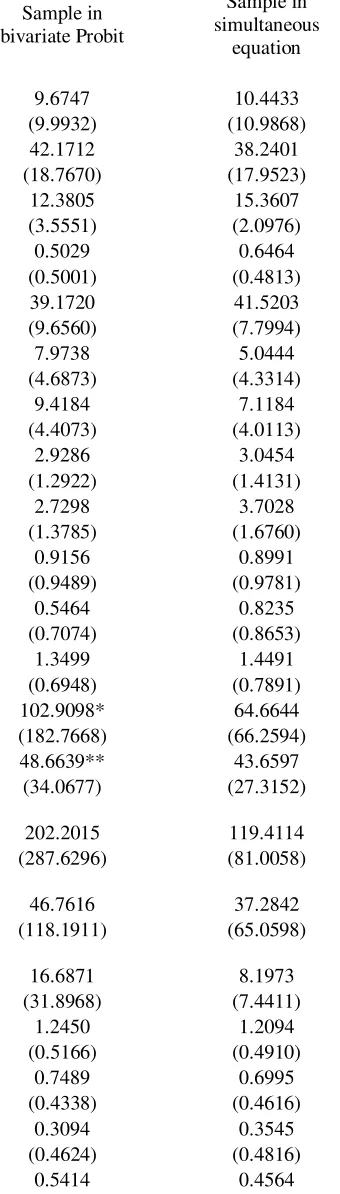
The following table shows descriptive statistics on all variables included in regressions. There are two columns; the first one includes only the observations which were included in Table 2 (a bivariate Probit estimation), and the second column includes those which were employed in tables 3 and 4 (an instrumental variables regression). Although the full sample is larger, its size decreased due to missing data.
Table 1. Descriptive Statistics
Sample in bivariate Probit
Sample in simultaneous
equation Variable name
Child's weekly hours of housework 9.6747 10.4433 (9.9932) (10.9868) Spouse's weekly hours of housework 42.1712 38.2401
(18.7670) (17.9523) Child's age 12.3805 15.3607
(3.5551) (2.0976) Fraction of male children 0.5029 0.6464
(0.5001) (0.4813) Spouse's age 39.1720 41.5203 (9.6560) (7.7994) Spouse's years of schooling 7.9738 5.0444
(4.6873) (4.3314) Head of household's years of schooling 9.4184 7.1184
(4.4073) (4.0113) # of adults in household 2.9286 3.0454
(1.2922) (1.4131) # children < 18 in household 2.7298 3.7028
(1.3785) (1.6760) # of children < 6 years old in household 0.9156 0.8991
(0.9489) (0.9781) # girls 11 – 17 years old in household 0.5464 0.8235
(0.7074) (0.8653) # adult women 18-55 years in household 1.3499 1.4491
(0.6948) (0.7891) Child's weekly earnings (in Peruvian Soles of 2000) 102.9098* 64.6644 (182.7668) (66.2594) Spouse's weekly earnings (in Peruvian Soles of 2000) 48.6639** 43.6597
(34.0677) (27.3152) Head of household's weekly earnings (in Peruvian
Soles of 2000) 202.2015 119.4114 (287.6296) (81.0058) Per capita weekly income from other household
members (in Peruvian Soles 2000) 46.7616 37.2842 (118.1911) (65.0598) Per capita weekly non labor income (in Peruvian
Soles of 2000) 16.6871 8.1973 (31.8968) (7.4411) # of floors in dwelling 1.2450 1.2094
(0.5166) (0.4910) Water connection inside dwelling 0.7489 0.6995
(0.4338) (0.4616) Material of Walls: Adobe 0.3094 0.3545
(0.4984) (0.5015) Dwelling in urban area 0.8011 0.7482
(0.3993) (0.4370) Child attends school? 0.9099 0.6163
(0.2865) (0.4896)
Number of observation 1681 75 Standard error in parenthesis
* Includes 151 observations only ** Includes 748 observations only
4. Results
4.1 Participation in the labour market
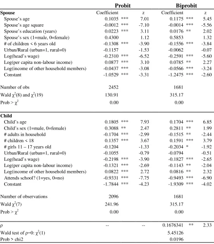
The first step is to estimate the bivariate Probit model for the participation of the spouse and child in the labour market. In each equation, I included variables related to individual characteristics such as age, sex, and education and variables that describe household characteristics such as wages, income, number of adults, and number of children younger than 18 years old. Since this is a stratified sample, weighted regressions were used.
variable has no effect on that participation13. It seems that households in which the head is a
[image:16.612.93.532.172.673.2]woman (and the spouse is male) do not behave differently than those in which the head is male and the spouse is a woman.
Table 2: Probit Estimation of Participation in Labour Market
Probit
Biprobit
Spouse Coefficient z Coefficient z
Spouse’s age 0.1035 *** 7.01 0.1175 *** 5.45 Spouse’s age square -0.0012 *** -7.10 -0.0014 *** -5.56 Spouse’s education (years) 0.0223 *** 3.11 0.0176 ** 2.02 Spouse’s sex (1=male, 0=female) 0.4300 1.12 0.5853 1.32 # of children < 6 years old -0.1308 *** -3.90 -0.1556 *** -3.84 Urban/Rural (urban=1, rural=0) -0.1157 -1.53 -0.0062 -0.07 Log(head’s wage) -0.2310 *** -6.52 -0.2591 *** -5.60 Log(per capita non-labour income) 0.0877 *** 3.10 0.0785 ** 2.27 Log(income of other household members) -0.0437 *** -3.08 -0.0566 *** -3.24 Constant -1.0529 *** -3.31 -1.2475 *** -2.60
Number of obs 2452 1681
Wald χ2(8) and χ2
(19) 130.91 315.17
Prob > χ2
0.00 0.00
Child
Child’s age 0.1805 *** 7.93 0.1704 *** 6.85 Child’s sex (1=male, 0=female) 0.3088 ** 2.47 0.2811 ** 1.99 # adults in household -0.1704 *** -2.99 -0.1515 ** -2.44 # children < 18 0.1357 *** 3.67 0.1591 *** 3.79 # girls 11 – 17 years old -0.1204 -1.33 -0.2034 * -1.92 Urban/Rural (urban=1, rural=0) -0.1055 -0.79 -0.0794 -0.51 Log(head’s wage) -0.2198 *** -3.90 -0.1827 *** -2.65 Log(per capita non-labour income) -0.1321 *** -2.69 -0.1143 ** -2.04 Log(income of other household members) 0.0822 *** 2.72 0.0816 ** 2.32 Attends school? (1=yes, 0=no) -0.9331 *** -7.75 -0.9493 *** -6.90 Constant -1.7844 *** -4.23 -1.9309 *** -4.02
Number of observations 2096 1681
Wald χ2
(7) 241.96 315.17
Prob > χ2
0.00 0.00
ρ -- -- 0.1676341 ** 2.33
Wald test of ρ=0: χ2
(1) 5.45126
Prob > chi2 0.0196 * significant at 10% level, ** significant at 5% level, *** significant at 1% level
13
In the case of child labour force participation, the older the child is, the more likely it is that he or she will participate in the labour market. There is also a greater level of participation for boys than girls. These two results agree with many empirical papers on child labour14. Also, the number of adults in the household reduces the probability of child participation. An explanation for this result is that more adults in a household means more individuals who can work, and the household will thus be able to “buy” more education and more leisure time for the child; consequently, we would observe less child labour. The number of girls of ages 11 – 17 also has a negative impact on the participation in the labour market. I expected an opposite sign, since girls usually work at home, and this affords more time to boys to work in the market.
Concerning the effect of the head of household’s wage, its coefficient is negative; non-labour income also has a negative effect on childhood participation, but the effect of the income of other members is positive. A possible explanation for the latter result is that if other members in the family (such as older siblings) work, the child may feel motivated to work as well. Finally, there is a negative relationship between school attendance and participation of children in the labour market.
Regarding the other parameters and statistics, the parameter , which is the correlation between the error terms in both equations in the bivariate Probit regression, is positive and significant. This means that whenever we observe a working spouse, it is more likely that we will also observe at least one working child in household, and this confirms that the bivariate Probit estimation is the correct method to use, rather than the standard Probit. The Wald statistic of joint significance of the variables shows that the model fits well.
4.2 Determinants of household work
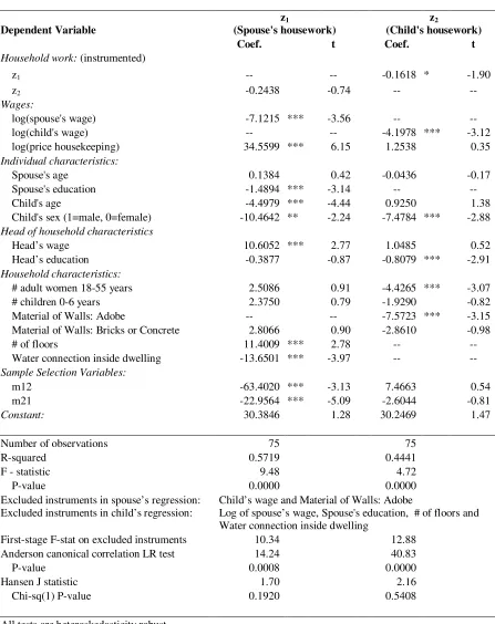
The second step involves estimating the model by the two-stage least-squares method and correcting for sample selection as described in section 2. Table 3 presents the results of the estimation of equations (8) and (9), in which all tests are heteroskedasticity robust.
14
Table 3: Determinants of the demand for household work
Dependent Variable
z1
(Spouse's housework)
z2
(Child's housework)
Coef. t Coef. t
Household work: (instrumented)
z1 -- -- -0.1618 * -1.90
z2 -0.2438 -0.74 -- --
Wages:
log(spouse's wage) -7.1215 *** -3.56 -- -- log(child's wage) -- -- -4.1978 *** -3.12 log(price housekeeping) 34.5599 *** 6.15 1.2538 0.35
Individual characteristics:
Spouse's age 0.1384 0.42 -0.0436 -0.17 Spouse's education -1.4894 *** -3.14 -- -- Child's age -4.4979 *** -4.44 0.9250 1.38 Child's sex (1=male, 0=female) -10.4642 ** -2.24 -7.4784 *** -2.88
Head of household characteristics
Head’s wage 10.6052 *** 2.77 1.0485 0.52 Head’s education -0.3877 -0.87 -0.8079 *** -2.91
Household characteristics:
# adult women 18-55 years 2.5086 0.91 -4.4265 *** -3.07 # children 0-6 years 2.3750 0.79 -1.9290 -0.82 Material of Walls: Adobe -- -- -7.5723 *** -3.15 Material of Walls: Bricks or Concrete 2.8066 0.90 -2.8610 -0.98 # of floors 11.4009 *** 2.78 -- -- Water connection inside dwelling -13.6501 *** -3.97 -- --
Sample Selection Variables:
m12 -63.4020 *** -3.13 7.4663 0.54 m21 -22.9564 *** -5.09 -2.6044 -0.81
Constant: 30.3846 1.28 30.2469 1.47
Number of observations 75 75 R-squared 0.5719 0.4441 F - statistic 9.48 4.72 P-value 0.0000 0.0000 Excluded instruments in spouse’s regression: Child’s wage and Material of Walls: Adobe
Excluded instruments in child’s regression: Log of spouse’s wage, Spouse's education, # of floors and Water connection inside dwelling
First-stage F-stat on excluded instruments 10.34 12.88 Anderson canonical correlation LR test 14.24 40.83 P-value 0.0008 0.0000 Hansen J statistic 1.70 2.16 Chi-sq(1) P-value 0.1920 0.5408
All tests are heteroskedasticity robust.
The sign of the derivative of z1 with respect to z2 is negative but not significant; the derivative of z2
with respect to z1 is also negative but significant. Theory says that a positive sign of this parameter
means the two labour inputs are complements, and that a negative sign corresponds to substitutes. Since both signs are negative, I suspect the fulfilment of the substitution hypothesis, but that evidence is not strong because one of the parameters is not significant.
In relation to the relationship between hours worked at home and market wages, Table 3 shows that there is a significant negative relationship between those variables in the two equations, and the parameters are significantly different from zero. In the case of the market price of
housekeeping services, the theory indicated that the relationship between household work and this price was positive. The results are consistent with this hypothesis in the first regression, but I cannot confirm that in the case of the child home labour equation, because the parameter is not significant.
Some of the individual characteristics affected the hours spent doing household work. The more educated the spouse was, the fewer hours the spouse worked at home. Also, the spouse’s age was not significant in either regression. In the case of the child’s characteristics, the age and sex variables affected the spouse’s hours of household work, but only the child’s sex affected the child’s household work. An older child in the household meant less housework for the spouse, but surprisingly, a male child in the house meant less housework performed by the spouse. On the other hand, older children participate more in housework than younger children, but the effect is not significant. It is also observed in Table 2 that girls work more at home than boys. These results are intuitive and expected.
The head of household characteristics also have an effect on the demand for household work. A higher head wage implies fewer hours of household work for a spouse. Also, a higher level of education for the head of a household is related to fewer hours of household work for a child.
residence. Some of them were included in one regression only for identification purposes. The number of adult women in a house decreases a child’s household work and increases the spouse’s work, but the latter is not significant. This result makes sense because in less-developed countries, women play an important role in household work. Perhaps those adults engage in household production, giving more time to children to study or play. Also, the presence of children from zero to six years of age decreased the hours of child housework, but the parameter is not significant. It is also not significant for a spouse’s housework.
Concerning house characteristics, the results show that in the case of “Material of Walls: Adobe”, the material reduces child housework compared to the rest of the categories: walls made of cane and mud, stone and mud, wood, matting, and others. In Peru, adobe walls are very common in poor rural houses in the sierra (highlands). In this area, children are used to working many hours outside the home, so it is reasonable that they have little time to spend at home doing housework. In contrast, walls made of bricks/concrete are common in cities in poor and non-poor areas. The effect on child housework is negative but not significant.
Something different occurs in the case of the number of storeys and the water connection inside the dwelling. They were included only in the spouse’s regression because they had no impact on child housework. A larger house with more floors implies more spousal housework, and a water connection inside the dwelling causes less spousal housework. This last result is intuitive, since a house with a water connection requires less work of a housekeeper to get the water the family needs.
The last group of variables in Table 3 is the group of sample selection variables that correct the double selection problem. They were significant in the spouse’s regression only. The set of goodness-of-fit statistics shows acceptable results, despite the low number of observations. The instruments selected passed the “rule of thumb” because the first-stage F statistic is greater than 10 in both equations, so they are relevant. The Anderson test rejects the null hypothesis of
4.3 Estimation of a household production function
It is interesting to obtain the technical parameters of the production function. One way to do it is to compare the parameters in equations (8) and (9) with those in (5) and (6) and then solve for the parameters . This is not difficult to do, but the standard errors have to be calculated by the delta method, which is not accurate here because of the low number of observations. Another weakness is that it is hard to impose a cross equation restriction in the estimation of equations (8) and (9) related to the equality of the second derivative 2f z1z2 2f z2z1. In terms of the parameter in (8) and (9), it is equivalent to impose the restriction2/11/1. An alternative way is to estimate equations (5) and (6) directly as a system by IV, which produces estimates of the parameters of equation (4), and the “composite” parameters b1 and b2. Additionally, it is easier to impose the cross-equation restriction mentioned above, which is in this case
simply 12 21. Therefore, I estimate (5) and (6) by 2SLS as a system taking z1 and z2 as endogenous and including the same group of variables and instruments in the regressions in Table 3, including the sample selection variables Mˆ12 and Mˆ2115.
These regressions permit one to test easily if there are differences in the production function when the child who works at home is boy or girl. We could think that the parameter 22 (which
represents the slope of the marginal return of child household work) may vary by sex. The next equation is an alternative specification of equation (7), where S is the dummy variable which equals 1 if the child is a boy and 0 if the child is a girl. The parameter 22 measures that gender effect.
P w z S z
z
b212 122 222( 2) 2 (14)
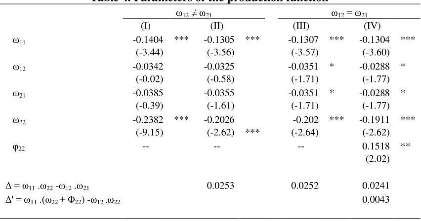
Table 4 shows the results for two regressions, with and without the cross-equation restriction. Column (I) shows the estimated parameters derived from the regressions in Table 3, whose
standard errors were calculated by the delta method. That column is the only one that shows robust
15
standard errors. The other three columns were estimated “as a system” in the way explained above. Column (II) also assumes that 12 21 and was estimated. We observe little change in the
estimates, but important changes in the calculated “t-ratios”. The last two columns assume that12 21, but the fourth one estimates (15) instead of (6). The parameters of all remaining control variables are not shown, but they were the same as those in Table 3.
As we see, the estimates are very similar in the restricted and unrestricted model because 12is very close to21 in the unrestricted model. The negative sign of the parameters 11 and 22 shows that the marginal products of labour are downward-sloping. The negative sign of ω12 is
[image:22.612.99.525.367.591.2]consistent with the hypothesis that labour inputs are substitutes. Furthermore, the sign of the determinant 11221221 is positive in all cases, which confirms that the production function is strictly concave because the matrix in equation (5) is negative definite.
Table 4. Parameters of the production function
ω12≠ ω21 ω12 = ω21
(I) (II) (III) (IV)
ω11 -0.1404 *** -0.1305 *** -0.1307 *** -0.1304 *** (-3.44) (-3.56) (-3.57) (-3.60)
ω12 -0.0342 -0.0325 -0.0351 * -0.0288 * (-0.02) (-0.58) (-1.71) (-1.77)
ω21 -0.0385 -0.0355 -0.0351 * -0.0288 * (-0.39) (-1.61) (-1.71) (-1.77)
ω22 -0.2382 *** -0.2026 -0.202 *** -0.1911 *** (-9.15) (-2.62) *** (-2.64) (-2.62)
φ22 -- -- -- 0.1518 ** (2.02)
Δ = ω11 .ω22 -ω12 .ω21 0.0253 0.0252 0.0241
Δ' = ω11 .(ω22 + Φ22) -ω12 .ω22 0.0043
t-ratios in parenthesis
* = significant at 10% level, ** = significant at 5% level, *** = significant at 1% level.
than that for girls (22). This result suggests that the technology is different when a boy or girl does the housework.
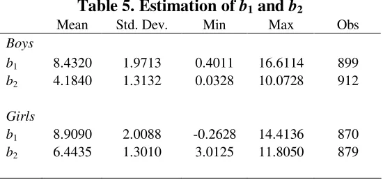
Finally, Table 5 shows the results of the predicted values of b1 and b2, which vary across individuals because they depend on the individual and household characteristics. The table has been divided in two. On top we see descriptive statistics on the predicted values of b1 and b2 when the child who does housework is a boy; on bottom we find the same statistics when the child is a girl. According to the economic theory, these predicted values should be strictly positive.
Fortunately, only one observation was negative, with a value close to zero.
[image:23.612.174.449.402.531.2]Concerning the results for b1 (a parameter of the spouse’s marginal product), there is little change whether the working child at home is boy or girl. On the other hand, b2 is smaller for boys than for girls. These estimates, along with the estimation of the's, tells us that girls are more productive at home than boys (at least up to some level).
Table 5. Estimation of b1 and b2
Mean Std. Dev. Min Max Obs
Boys
b1 8.4320 1.9713 0.4011 16.6114 899
b2 4.1840 1.3132 0.0328 10.0728 912
Girls
b1 8.9090 2.0088 -0.2628 14.4136 870
b2 6.4435 1.3010 3.0125 11.8050 879
From the results of the fourth column in Table 4 and those in Table 5, I have simulated the
Finally, Figure 3 shows the marginal product curves for boys and girls, taking the average value of
1
b , b2 andz1. The graph shows that both curves are downward-sloping, and that girls are more productive than boys in the range of zero to 15 hours of household work per week. Beyond that point, boys have a higher marginal product.
I propose two possible explanations for the latter result. One could be related to natural differences between boys and girls when it comes to do housework. Another more plausible explanation says that the observed difference in productivity could be the result of previous training in house chores, which could be the result of cultural differences16. Thus, if girls are trained to do housework since an early age, they would be more productive than boys due to human capital accumulation.
16
5. Summary and Conclusions
Unlike other papers on child labour time allocation, this paper estimates the determinants of a child’s household work, stressing the role of its wage and the wages of other family members.
The results showed that the hours that individuals spend on household work depend negatively on their respective wages, and there are signs that the two inputs are substitutes. Additionally, hours spent on household work depend on individual characteristics like sex, age, head of household’s education and household characteristics. However, one shortcoming of these estimations is that the number of selected observations is very small compared to the total sample.
Finally, the parameters of the quadratic home production function were estimated. The results are consistent with a strictly-concave production function. The estimates confirm that a child’s household work and a spouse’s household work are substitutes for each other. Besides, the isoquants show that when girls work at home, fewer hours of work are required to produce the output, and the graph of marginal products shows that girls are more productive than boys in the range of zero-to-15 hours per week, although the productivity of girls declines faster than that of boys.
References
Becker, Gary S. (1965). “A theory of the allocation of time.” The Economic Journal 75, no. 299: 493-517.
Bhalotra, Sonia. (2001). Is child work necessary? Social Protection Discussion Paper Series. Washington, D.C.: World Bank.
Binder, Melissa and David Scrogin. (1999). “Labor force participation and household work of urban schoolchildren in Mexico: characteristics and consequences.” Economic Development and Cultural Change, 48, no.1: 123-154.
Birdsall, Nancy and Susan E. Cochrane. (1982). “Education and parental decision making: a two generation approach.” In Education and Development, ed. Anderson Lascelles and Douglas M. Windham, . Lexington Mass.: Lexington Books, D.C. Heath and Company.
Brown, Drusilla K., Alan V. Deardorff and Robert M. Stern. (2003). “U.S. trade and other policy options and programs to deter foreign exploitation of Child Labor”. Discussion paper 99-04, Medford, M.A.: Tufts University, Department of Economics.
DeGraff, Deborah S., Richard E. Bilsborrow. (2003). “Children’s school enrollment and time at work in the Philippines.” Journal of Developing Areas 15, no.1: 127-158.
Fishe, Raymond P.H., R.P. Trost and Philip M. Lurie. (1981). “Labor force earnings and college choice of young women: an examination of selectivity bias and comparative advantage”. Economics of Education Review 1, no. 2: 169-191.
Garcia, Luis. (2006). “Child labor, home production and the family labor supply”. Revista de Analisis Economico 21, no.1: 59-79.
Gronau, Reuben. (1977). “Leisure, home production, and work – the theory of the allocation of time revisited.” Journal of Political Economy 85, no.6: 1099-1123.
Kerkhofs, Marcel and Peter Kooreman. (2003). “Identification and estimation of a class of household production models.” Journal of Applied Econometrics 18: 337-369.
Kotz, Samuel; N. Balakrishna and Norman L. Johnson. (2000). Continuous Multivariate Distributions: Volume 1: Models and Applications. New York: Wiley.
Lee, Lung-Fei, G.S. Maddala and R.P. Trost. (1980). “Asymptotic covariance matrices of two-stage probit and tobit methods of simultaneous equations models with selectivity.” Econometrica 48, no. 2: 491-504.
Levison, Deborah and Karine S. Moe. (1998). “Household work as a deterrent to schooling: an analysis of adolescent girls in Peru.” Journal of Developing Areas 32 (Spring): 339-356. Maddala, G.S. (1983). Limited-Dependent and Qualitative Variables in Econometrics. New York:
Cambridge University Press.
Newman, John L. and Paul J. Gertler. (1994). “Family productivity, labor supply and welfare in a low income country.” Journal of Human Resources 29, no. 4. Special Issue: The family and intergenerational relations (Autumn): 989-1026.
Ransom, Michael M. (1987). “An empirical model of discrete and continuous choice in family labor supply.” The Review of Economics and Statistics 69, no. 3: 465-472.
Skoufias, E. (1994). “Market wages, family composition and the time allocation of children in agricultural households.” Journal of Development Studies 30: 335-360.