What does the eclectic trade model say about the Samuelson conundrum?

Lancaster University Management School

Working Paper

2006/035

What does the eclectic trade model say about the Samuelson

conundrum?

Kwok Tong Soo

The Department of Economics Lancaster University Management School

Lancaster LA1 4YX UK

© Kwok Tong Soo

All rights reserved. Short sections of text, not to exceed two paragraphs, may be quoted without explicit permission,

provided that full acknowledgement is given.

What does the eclectic trade model say about the

Samuelson conundrum?

Kwok Tong Soo

Lancaster University

December 2005

Abstract

Can growth of a trading partner harm a country? This paper seeks to

an-swer this question through the use of an eclectic trade model which is similar

in ‡avour to Markusen (1986). This paper makes two contributions. First,

it develops a simple and tractable model of international trade based on a

combination of imperfect competition, comparative advantage, and identical

but non-homothetic preferences in a three country framework. Second, it

uses this framework to consider the possibility of losses from partner-country

growth in a free-trading environment. We …nd that the presence of

nonhomo-thetic preferences in particular, leads to a home bias in consumption which

dampens any negative welfare e¤ects when a country’s trading partners grow.

JEL codes: F12, F14.

Keywords: International trade; three countries; non-homothetic preferences.

Thanks to Holger Breinlich, Dimitra Petropoulou, Julia Shvets and seminar participants at Lancaster University, Universiti Malaya and the European Trade Study Group 2005 in Dublin for valuable comments and suggestions. The usual disclaimer applies.

y_{Correspondence: Department of Economics, Management School, Lancaster University,}

1

Introduction

Since the early 1990s, China and India have emerged as the fastest-growing economies in the world. Their rapid growth has inspired much debate and speculation in the media. For example, analysts at Goldman Sachs (Wilson and Purushothaman (2003)) predict that China, the US and India will be the three largest economies in the world by 2050. This growth in China and India has been fueled by an outward-orientated economic policy, which has seen export growth in both countries of over 10 percent per year since the 1980s.

This rapid growth has led to fears especially in the US, that China and India may threaten the livelihood of the people in the developed countries. This sense of a threat is compounded by recent policy incidents, for example the US tari¤ on steel imports in 2002 and the EU’s quota restriction on textile imports in 2005. These fears were given academic support in Samuelson’s (2004) Journal of Economic Perspectives paper, as well as in an earlier Journal of Economic Literature paper (Samuelson (2001)), which argued that in a simple Ricardian model of trade based on technological di¤erences across countries, the US may lose from economic growth in China if China becomes more similar to the US in terms of its comparative advantage. This is what we refer to as the Samuelson conundrum: that a country can be made worse o¤ by changes that occur in its trading partner(s). It poses a conundrum because it is demonstrably true in the context of the model that Samuelson (2004) sets out, yet at the same time appears to ‡y in the face of trade economists’gains from trade result.

In an extended discussion section, Samuelson (2004) argues that the insight from his simple model can be generalised to richer models. This paper sets out to perform this generalisation. We develop a three-country model based on increasing returns to scale at the level of the …rm and monopolistic competition, combined with di¤erences in relative factor endowments and technology across countries, and non-homothetic preferences. In the interest of keeping the model as simple as possible, we impose strong assumptions on the technology side along the lines of Krugman (1981), and we adopt the simplest possible, quasi-linear utility function. The underlying monopolistic competition model is that of Krugman (1980), based on the Dixit-Stiglitz (1977) framework.

In addition to considering Samuelson’s result in a more general framework, this paper also represents a step forward in developing the eclectic approach of Markusen (1986). In particular, our setup is much more tractable than Markusen (1986) yet re-tains much of the same ‡avour. Our three-country framework also di¤ers from that of Markusen (1986) as here our three countries may be di¤erent from one another, whereas Markusen (1986) focussed on pairs of countries, where countries within each pair are symmetric to one another. Also, of our three countries, we assume that two of them are less-developed countries while the third represents a developed country. This then allows us to explore what happens for example to the rest of the developing world as China and India experience rapid economic growth. The use of nonhomothetic preferences in economic models has a long history, dating back to Linder’s (1961) work on international trade between rich and poor countries, and has received empirical validation in Hunter (1991) who showed that nonhomothetic preferences may account for as much as one quarter of interindustry trade ‡ows. More recent empirical evidence by Chung (2002) and Dalgin, Mitra and Trindade (2005) con…rms the importance of demand nonhomotheticity in international trade.

inter-country rather than intra-inter-country interactions.

Our main …nding is that the introduction of nonhomothetic preferences and love-for-variety coupled with increasing returns, leads to additional channels through which the e¤ects of changes in a trading partner a¤ect a country, in addition to the terms of trade e¤ect identi…ed by Samuelson (2004). First, nonhomothetic preferences generate a home bias in demand despite the absence of transport costs, as the developed country, being relatively abundant in high-wage, high-skill workers, will also have a greater relative demand for high-income-elasticity goods such as electronics which are produced by high-skill workers. As a result, the developed country is insulated to a certain degree from changes in the developing countries.

Second, as the developing countries grow, the increased supply of goods also implies a larger number of varieties available for consumption. Therefore, whilst growth in a developing country may improve or worsen the developed country’s terms of trade through its impact on world relative supply, there will also be a gain from more varieties because of love-for-variety in consumption, which dampens any negative terms of trade e¤ects of growth in the developing country. Whilst our numerical examples in Section 3 show that the developed country never experiences a welfare loss from the changes in the developing countries, we see these results not as de…nitive, but rather as indicative of the forces at work.

The model we present in this paper relates to several strands of literature. As it uses a monopolistic competition model, it builds on the insights from Helpman and Krugman (1985). In generating a gravity-type prediction on the volume of trade, it follows work by Anderson (1979) and Krugman (1979, 1980). And …nally, in discussing international trade between developed and less developed countries, it is related to the work by Markusen (1986), Flam and Helpman (1987), Stokey (1991), Ramezzana (2000), Matsuyama (2000), Mitra and Trindade (2005), and Chung (2003), among others.

2

The model

In this section we …rst describe the autarkic equilibrium of the model, then consider its implications for free trade in goods but not in labour.

2.1

Autarkic equilibrium

The basic setup of the model is that of a monopolistic competition model developed from Krugman (1981), with the main points of departure being the use of non-homothetic preferences and a three-country setup. There are three countries z = 1;2;3, and two industries h = 1;2. Each industry consists of a large number of products which enter symmetrically into demand. The representative consumer has the following quasi-linear utility function:

U = lnC1+C2 (1)

where each ofCh is a composite index of products comprising a

constant-elasticity-of-substitution (CES) function:

C1 = P

ic1i C2 =

P

jc2j 0< <1 (2)

where c1;i is consumption of the ith product of industry 11 and so on2. The value

of measures the degree of substitutability among products within an industry. The lower is , the more di¤erentiated are products in the industry. Quasi-linear utility implies that consumption of products in both industries initially increases with income, then products in industry 1 have zero income elasticity of demand above a certain income threshold, beyond which all additional income is spent on products in industry 2. We assume that consumer income always lies beyond this threshold. Beyond this threshold, this function is also quasi-homothetic, so that

1_{A note on terminology: we use goods and industries interchangeably to indicate broad}

in-dustry groups, and products and varieties interchangeably to indicate within-inin-dustry varieties.

2_{This formulation of the CES function is slightly di¤erent from the standard one used in}

shifting income between agents does not change the total expenditure on di¤erent industries. This allows us to aggregate individual demands.

Each industry is produced using a speci…c type of labour, so that there are two types of labour y = 1;2. Type 1 labour is used in industry 1 and type 2 labour in industry 2. Making the labour industry-speci…c prevents us from considering the redistribution of labour across industries as parameter values change; however it does make the model much easier to solve, and in any case sectoral reallocation of labour is not the main focus of the present paper. There is also substantial evi-dence that factors of production are not very mobile across sectors; see for example Wacziarg and Wallack (2004) or Lee and Wolpin (2004). Labour is not speci…c to products within each industry. The cost function for any product in each industry exhibits increasing returns to scale:

l1i = + x1i l2j = + x2j i= 1; :::; n1 j = 1; :::; n2 (3)

where l1i is labour used in producing the ith product of industry 1, x1i is the

output of that product and so on. Because of increasing returns to scale, consumers’ preference for variety, and the large number of potential products of each industry, each …rm will produce its own unique product.

Total employment in each industry is equal to the sum of employment in each product in that industry. Full employment is assumed. The labour force is exoge-nously split between the two types of labour. In country 1, the split is as follows:

P

il

1 1i =L

1

1 = 1 1

P

jl

1 2j =L

1

2 = 1 1; 1 >0 1 2 1 (4)

whereLz_y is the total endowment of labour type y in country z. The parameters and measure the quantity of the di¤erent types of labour. The second constraint on the parameter values indicates that country 1 has more type 1 labour than type 2 labour. This restriction will be dropped when we consider economic growth later on; the present notation is extremely ‡exible and will allow us to consider changes in the three countries without having to introduce additional notation.

1

1 , the …rm’s pro…t-maximising price is a constant markup over marginal cost:

p1i =

w1

p2j =

w2

(5)

wherep1i is the price of product i in industry 1 and so on.

Free entry and exit of …rms ensures that pro…ts are zero in equilibrium. Com-bining this zero pro…t condition and the …rms’ pricing decision allows us to solve for the output (and hence size) of each …rm:

x1i =x2j =

1 =x (6)

Notice that …rm sizes are independent of market size. Then the number of …rms in each industry can be obtained by combining the full employment condition with the labour endowment and the size of …rms:

n1 = 1 1

+ x n2 =

1

+ x (7)

The number of …rms is proportional to the labour endowment. Relative prices and wages are determined from the …rst order conditions of the consumer’s maximisation problem:

P

ic1i

1

c_1i 1 = p1i c2j1 = p2j

where is the Lagrange multiplier on the budget constraint or the marginal utility of income. Given our symmetry assumptions, the relative prices are:

p2j

p1i

=n1c1i (8)

Equilibrium wages are determined by these prices and the pricing equation (5).

2.2

Free trade equilibrium

is given in the previous subsection. Assume that countries 2 and 3 have the following endowments:

Country 2 : P_il₁2_i =L2₁ = _{2 2} P_jl₂2_j =L2₂ = ₂ (9)

Country 3 : P_il₁3_i =L3₁ = ₃ P_jl₂3_j =L3₂ = _{3 3}

2; 2; ; 3; 3 >0 2 2 2 3 2 3

where as aboveLz

y is the total endowment of labour typey in countryz. The

para-meters and measure the similarity of relative endowments across the countries. For example, if _z = 0 for all countries z, then each country has only one type of labour and hence can only produce varieties of a single industry. If _z = _{z z}, all countries have the same relative endowment ratio. Each country’s total endowment is given by z.

Given the relationship between the endowment parameters and , countries 1 and 2 are relatively well-endowed with type 1 labour compared to country 3. Therefore, Countries 1 and 2 have a comparative advantage in industry 1 and Country 3 in industry 2. Total world endowment of type 1 labour is equal to

( _{1 1}+ _{2 2}+ ₃) while the total world endowment of type 2 labour is equal

to( _{3 3}+ ₁+ ₂).

In this model, changes in endowments and changes in technology are identical in their e¤ects on production but not on their e¤ects on consumption. For example, whilst doubling total endowments may be caused either by a doubling of the number of workers, a doubling of labour productivity, or some combination of the two, changing the number of workers would a¤ect the demand for industry 1, because of our nonhomothetic preferences, whereas changing labour productivity would not have any impact on the demand for industry 1, as any additional income will be spent entirely on industry 2. For the remainder of the paper we hold the number of workers constant and identical across countries and allow productivity to vary across countries; therefore, the labour endowments de…ned above should be interpreted as e¢ ciency units of labour.

1 and 2, with a comparative advantage in low income elasticity of demand goods such as food and clothing3 which are produced using unskilled labour. Our speci…-cation allows us to introduce superior technology in the developed countries relative to the less developed countries.

Since preferences are identical across countries, the pro…t maximising price is the same as in equation (5) above. From the …rst order conditions for the consumer’s problem above, equilibrium price ratios are:

p2j

p1i

=nW₁ c_1i (10)

wherenW₁ is the total number of type 1 …rms in the world. We normalisep1 =w1 = 1

which implies = . Prices and wages in industry 2 are pinned down by equation (10). Free trade in goods implies factor price equalisation across countries, measured in e¢ ciency units of labour.

From equations (7) and (6), and making use of the assumption that = , the total world output of each industry is:

nW₁ x= _{1 1}+ _{2 2}+ ₃ nW₂ x= _{3 3}+ ₁+ ₂

National incomes Yz _{are equal to:}

Y1 = _{1 1}+w_{2 1} Y2 = _{2 2}+w_{2 2} Y3 = ₃+w2( 3 3)

Because of the quasi-linear utility function and identical numbers of consumers in each country, each country consumes one-third of the world output of each product of industry 1; that is, total expenditure on industry 1 (and total consumption, given our normalisation above) in each country is equal to 1 1+ 2 2+ 3

3 . Therefore, we

can back out the total expenditure by each country on industry 2 by subtracting expenditure on industry 1 from national income. Appendix A provides details of this calculation.

De…ning X_hzv as the exports of industry h from country z to country v, we can compute the exports of each country to the other two countries. Because all varieties of a good are symmetric, a country’s exports of an industry to another country is equal to the output of the country in that industry multiplied by the fraction of

world output that is consumed in the importing country. For country 1, exports of the two industries to countries 2 and 3 are:

X₁12=X₁13= 1 1

3 X 12 2 = 1 nW 2 x

E₂2 X₂13= 1

nW

2 x

E₂3 (11)

where Ez

y is the expenditure in country z of industry y as de…ned in Appendix

A. Therefore, country 1 exports the same quantity of industry 1 to both countries because of the quasilinear utility and the assumption of identical numbers of con-sumers in each country, but exports of industry 2 to the two countries are di¤erent because national expenditures on industry 2 are determined by national per capita incomes. Country 2’s exports to countries 1 and 3 can be obtained analogously.

X₁21=X₁23= 2 2

3 X 21 2 = 2 nW 2 x

E₂1 X₂23= 2

nW

2 x

E₂3 (12)

Country 3’s exports to countries 1 and 2 are:

X₁31=X₁32= 3

3 X 31 3 = 3 3 nW 2 x

E₂1 X₃32= 3 3

nW

2 x

E₂2 (13)

Our primary focus is on the welfare implications of changes in the parameter values for the three countries, but here we brie‡y comment on the observed trade patterns. Given the parameter restrictions we impose on the endowments, we can see that countries 1 and 2 export more of good 1 relative to good 2 than country 3. This is as expected, since the parameter restrictions mean that countries 1 and 2 are well-endowed with type 1 labour relative to country 3. Similarly, country 3 exports more of good 2 relative to good 1 compared to the other countries. There is also signi…cant bilateral trade within the same industry groups. This comes from the love-for-variety, monopolistic competition setup; with no trade barriers across countries, consumers will wish to consume identical amounts of each variety of each good, irrespective of the country of origin of the variety.

consump-tion. These are as we would expect, and are in line with the results from Krugman (1981).

3

Economic growth in the developing world

One of the main economic trends in the world today is the rapid economic growth of China and India. More generally, the world consists of developed countries and developing countries. Some of the latter countries are experiencing rapid economic growth whilst others in this category are not. This section makes use of the ‡exible framework developed in the previous section to explore the welfare implications of various types of growth on the di¤erent groups of countries.

We assume that national welfare is simply the sum of individual welfare, mak-ing use of the quasi-homotheticity of the utility function to allow for aggregation across individuals with di¤erent income levels. Due to the many interactions in the model, we focus on graphical representation of the results. It turns out that for the parameters we use below, in free trade good 2 always has a higher price than good 1 as a result of it being the income-elastic good. This also implies higher wages of type 2 labour as compared to type 1.

3.1

Analysis

identical so that only the welfare of country 2 is visible).

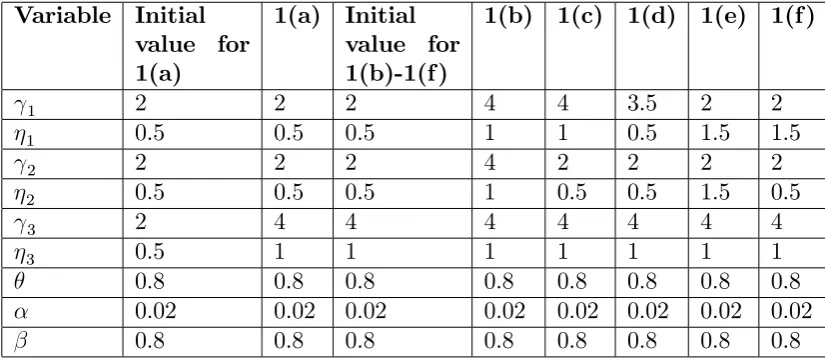
Given the assumption that country 3 is technologically superior to countries 1 and 2, we can explore what happens to welfare in the three countries when several things happen, holding country 3 unchanged:

1. Technological improvement in countries 1 and 2 in both sectors; technological catch-up with country 3 (Figure 1(b))

2. Technological improvement only in country 1 in both sectors (Figure 1(c))

3. Technological improvement in only one sector of country 1 (here, consider sector 1 of country 1) (Figure 1(d))

4. Countries 1 and 2 experience a change in endowments through a shift from type 1 labour (unskilled) to type 2 labour (skilled); endowment convergence with country 3 (Figure 1(e))

5. Endowment convergence of only country 1 to country 3 (Figure 1(f))

Figures 1(b) to 1(f) show all of these changes. Table 1 lists the parameter values for which each …gure is drawn; the column headings correspond to …nal parameter values for each …gure. What is immediately obvious from these …gures is that country 3 (the developed country) never experiences a welfare loss regardless of what happens in the two developing countries. This result holds for many alternative parameter values, but we do not wish to argue that this is a general result; rather, we use this …nding to explore the economic forces at work.

Intuitively, if the change in countries 1 and 2 imply expansion of world relative supply of good 1, this is a gain to country 3 as it is a net importer of this good, so its consumers bene…t from lower relative prices of imports. On the other hand, if the change in countries 1 and 2 imply expansion of world relative supply of good 2, this bene…ts country 3 as well because it remains the largest consumer of good 2 due to its high per capita income, and expanded world supply of good 2 increases the number of varieties of good 2 available, hence raising consumer welfare even whilst its terms of trade erodes as a result of this growth in countries 1 and 2.

as does a shift towards greater endowments of factors which yield output which have high income elasticity of demand.4 In addition, in the …gures, if only one developing country grows (country 1 in every case) and the other (country 2) does not, the country that does not grow also experiences a welfare improvement, albeit a marginal one.

This improvement in the welfare of country 2 when country 1 grows arises be-cause, if the change in country 1 is such that world relative supply of good 1 increases (e.g. as a result of technological improvement in sector 1, case 3 above or Figure 1(d)), the welfare gain from the increase in the number of varieties of good 1 available for consumption outweighs the welfare loss from the fall in the relative price of good 1. On the other hand, if the change in country 1 increases world supply of good 2 and decreases world supply of good 1, then it turns out that the gain in welfare from country 2 consumers consuming more of good 2 outweighs the loss of welfare from the lower consumption of good 1, as a result of the quasi-linear preferences which place a greater weight on consumption of good 2. There is also a gain from the increased number of varieties of good 2 available for consumption.

Therefore, there are essentially three forces at work in determining the welfare e¤ects of any change in the three countries. First, each of the changes leads to a change in world relative supply of the two goods. This a¤ects world relative prices and hence real incomes of each of the three countries. Second, there is the nonhomothetic utility function which leads to a home bias in consumption since less developed countries are relatively abundant in factors of production which are used in producing goods with low income elasticity of demand, and these countries also demand relatively more of the income-inelastic goods, because of their relatively low per capita income. The third force at work is the love of variety in consumption. An increase in world supply of a good, implies an increase in the number of varieties available for consumption, which raises welfare even in the face of declining real income. The second and third forces act to dampen any possible terms of trade losses from changes in a country’s trading partners.

4_{Immiserising growth of the Bhagwati (1958) type does not occur, because no country’s o¤er}

4

Discussion and Conclusions

Can the growth of a trading partner harm a country? This paper seeks to answer this question by developing a model of international trade between three countries that takes into account elements of factor endowment di¤erences across countries, intra-industry trade of the Dixit-Stiglitz type, and non-homothetic preferences. Al-though the model seeks to capture all of these important features of international trade, the use of simple and ‡exible functional forms allows us to consider several di¤erent ways in which countries can grow, and how this growth impacts on the welfare of both the growing country and its trading partners. Our key result is that the additional elements of our model relative to Samuelson (2004) generate a home bias in demand (from nonhomothetic preferences) and a new channel through which countries gain from trade (from love-for-variety). These additional e¤ects serve to dampen any negative e¤ects on a country of economic growth in its trading part-ners. Depending on the parameter values, it may even be the case that countries can never lose from growth in their trading partners.

Comparing our results to those of Samuelson (2004), when the trading partner experiences technological improvement in Samuelson’s (2004) model in the home (developed) country’s import-competing good, this harms the home country because it makes countries more similar and hence reduces the gains from trade which arise from di¤erences across countries. This does not happen in our model, because the developed country, having a higher per-capita income, also demands more of the good which uses intensively its abundant factor. Therefore, when its trading partners become more similar to it in terms of endowments, the developed country actually gains from this change because its consumers bene…t from having more varieties of the good at lower prices due to the increased supply.

developed country acquires more of type 2 labour. In this case, the developed coun-try clearly loses, as its endowment mix shifts towards the low-wage type 1 labour, reducing national income.

The additional elements of our model improve the implications of developing country growth on developed country welfare. However, as Jones and Ru¢ n (2005) note, what may be of concern to governments might not be absolute welfare and income levels, but welfare and income levels relative to those of other countries. Economic growth in less developed countries leads to a narrowing of the relative income gap between rich and poor countries, hence may be a cause for concern in rich countries even if their absolute welfare increases at the same time.

The use of an explicit three-country framework is also a relatively new develop-ment in a …eld that has been largely driven by two-country frameworks5. In this case, a three-country approach enables us to explore the interdependencies between countries when their trading partners grow. There exists the possibility of con‡ict between countries, as changes in one country may impact on other countries in di¤erent ways depending on the structure of each country’s economy. This again appears to be consistent with the con‡icts in international trade that have been observed between di¤erent countries.

5_{See for instance Markusen and Venables (2004) for a discussion of the limitations of the}

5

Appendix A: National expenditures on good 2

This Appendix provides the algebraic expressions for the national expenditures on good 2. De…ne national expenditure of country z on industry 2, Ez

2 as national

income less expenditures on industry 1. Then, this may be written as:

E₂1 = Y1 E₁1 = _{1 1} +w_{2 1} 1 1+ 2 2 + 3

3

= 1

3f2 1 2 1 2+ 2 3+ 3w2 1g

E₂2 = Y2 E₁2 = _{2 2} +w_{2 2} 1 1+ 2 2 + 3

3

= 1

3f2 2 2 2 1+ 1 3+ 3w2 2g

E₂3 = Y3 E₁3 = ₃+w2( 3 3)

1 1+ 2 2+ 3 3

= 1

References

[1] Anderson, James E. (1979), "A Theoretical Foundation for the Gravity Equa-tion",American Economic Review, 69(1): 106-116.

[2] Bhagwati, Jagdish N. (1958), "Immiserizing Growth: A Geometrical Note",

Review of Economic Studies, 25(3): 201-205.

[3] Bhagwati, Jagdish N., Arvind Panagariya and T. N. Srinivasan (1998),Lectures

on International Trade, 2nd edition, Cambridge, MA, MIT Press.

[4] Chung, Chul (2002), "Nonhomothetic Preferences and the Home Market E¤ect: Does Relative Market Size Matter?", mimeo, Georgia Institute of Technology.

[5] Chung, Chul (2003), "Factor Content of Trade: Nonhomothetic Preferences and "Missing Trade"", mimeo, Georgia Institute of Technology.

[6] Dalgin, Muhammed, Devashish Mitra and Vitor Trindade (2003), "Inequality, Nonhomothetic Preferences, and Trade: A Gravity Approach", mimeo, Uni-versity of Missouri.

[7] Dixit, Avinash K. and Joseph E. Stiglitz (1977), "Monopolistic Competition and Optimum Product Diversity", American Economic Review, 67(3): 297-308.

[8] Flam, Harry and Elhanan Helpman (1987), "Vertical Product Di¤erentiation and North-South Trade", American Economic Review, 77(5): 810-822.

[9] Fujita, Masahisa, Paul Krugman and Anthony Venables (1999), The Spatial

Economy, Cambridge, MA, MIT Press.

[10] Helpman, Elhanan and Paul R. Krugman (1985),Market Structure and Foreign

Trade, Cambridge, MA, MIT Press.

[11] Hunter, Linda (1991), "The Contribution of Nonhomothetic Preferences to Trade", Journal of International Economics, 30(3-4): 345-358.

[12] Johnson, Harry G. (1954), "Increasing Productivity, Income-Price Trends and the Trade Balance", Economic Journal, 64(255): 462-485.

[13] Johnson, Harry G. (1955), "Economic Expansion and International Trade",

[14] Jones, Ronald W. and Roy J. Ru¢ n (2005), "International Technology Trans-fer: Who Gains and Who Loses?", forthcoming, Review of International

Eco-nomics.

[15] Krugman, Paul R. (1979), "Increasing Returns, Monopolistic Competition, and International Trade", Journal of International Economics, 9(4): 469-479.

[16] Krugman, Paul R. (1980), "Scale Economies, Product Di¤erentiation, and the Pattern of Trade", American Economic Review, 70(5): 950-959.

[17] Krugman, Paul R. (1981), "Intraindustry Specialization and the Gains from Trade", Journal of Political Economy, 89(5): 959-974.

[18] Lee, Donghoon and Kenneth I. Wolpin (2004), "Intersectoral Labor Mobility and the Growth of the Service Sector", forthcoming,Econometrica.

[19] Linder, Ste¤an Burenstam (1961), An Essay on Trade and Transformation, New York, Wiley.

[20] Markusen, James R. (1986), "Explaining the Volume of Trade: An Eclectic Approach",American Economic Review, 76(5): 1002-1011.

[21] Markusen, James R. and Anthony J. Venables (2004), "A Multi-Country Ap-proach to Factor-Proportions Trade and Trade Costs", mimeo, London School of Economics.

[22] Matsuyama, Kiminori (2000), "A Ricardian Model with a Continuum of Goods under Nonhomothetic Preferences: Demand Complementarities, Income Distri-bution, and North-South Trade",Journal of Political Economy, 108(6): 1093-1120.

[23] Mitra, Devashish and Vitor Trindade (2005), "Inequality and Trade",

Cana-dian Journal of Economics, 38(4).

[24] Panagariya, Arvind (2004), "Why the Recent Samuelson Article is NOT about O¤shore Outsourcing" mimeo, Columbia University.

[26] Samuelson, Paul A. (2001), "A Ricardo-Sra¤a Paradigm Comparing Gains from Trade in Inputs and Finished Goods", Journal of Economic Literature, 39(4): 1204-1214.

[27] Samuelson, Paul A. (2004), "Where Ricardo and Mill Rebut and Con…rm Argu-ments of Mainstream Economists Supporting Globalization", Journal of

Eco-nomic Perspectives, 18(3): 135-146.

[28] Stokey, Nancy L. (1991), "The Volume and Composition of Trade Between Rich and Poor Countries",Review of Economic Studies, 58(1): 63-80.

[29] Wilson, Dominic and Roopa Purushothaman (2003), "Dreaming with BRICs: The Path to 2050", Goldman Sachs Global Economics Paper No. 99.

Variable Initial value for 1(a)

1(a) Initial value for 1(b)-1(f )

1(b) 1(c) 1(d) 1(e) 1(f )

1 2 2 2 4 4 3.5 2 2

1 0.5 0.5 0.5 1 1 0.5 1.5 1.5

2 2 2 2 4 2 2 2 2

2 0.5 0.5 0.5 1 0.5 0.5 1.5 0.5

3 2 4 4 4 4 4 4 4

3 0.5 1 1 1 1 1 1 1

0.8 0.8 0.8 0.8 0.8 0.8 0.8 0.8 0.02 0.02 0.02 0.02 0.02 0.02 0.02 0.02 0.8 0.8 0.8 0.8 0.8 0.8 0.8 0.8

Figure 1(a): Doubling country 3 labour productivity 0 1 2 3 4 5 6 7 Before After U tility u1(a) u2(a) u3(a)

Figure 1(b): Doubling country 1 and 2 productivity

0 1 2 3 4 5 6 7 Before After Utility u1(b) u2(b) u3(b)

Figure 1(c): Doubling country 1 labour productivity 0 1 2 3 4 5 6 7 Before After Utility u1(c) u2(c) u3(c)

Figure 1(d): Doubling country 1 productivity in good 1

0 1 2 3 4 5 6 7 Before After Utility u1(d) u2(d) u3(d)

Figure 1(e): Country 1 and 2 endowments become identical

to country 3

0 1 2 3 4 5 6 7 Before After Utility u1(e) u2(e) u3(e)

Figure 1(f): Country 1 endowments become identical

to country 3

0 1 2 3 4 5 6 7 Before After Utility u1(f) u2(f) u3(f)