Formation of Ravi Vallis outflow channel, Mars:morphological development, water discharge, and duration estimates

Formation of Ravi Vallis outflow channel, Mars:

Morphological development, water discharge,

and duration estimates

Harald J. Leask,1Lionel Wilson,1and Karl L. Mitchell1,2

Received 3 August 2005; revised 30 November 2005; accepted 16 December 2005; published 13 June 2006.

[1] We infer that the morphology of the Ravi Vallis channel system is consistent with it

having been eroded by water in a single flood event, and we have used the topography of the channel system to estimate the depth of water in the channel at various stages during its development. Values lie in the range 50– 150 m. Measured bed slopes, estimated water depths, and corresponding channel widths are used to obtain mean water flow speeds and volume flow rates. Water flow speeds are found to lie in the range

10– 25 m s1, and the discharge estimates vary from a maximum volume flux of30

106m3s1just after the start of the flood to less than 10106m3s1in the late stages. Using assumptions about the sediment-carrying capability of the water, estimates are obtained for the minimum duration of the water release event, the minimum total volume of water involved, and the crustal erosion rate. The duration is inferred to have been between 2 and 10 weeks, and the minimum total water volume was between 11,000 and 65,000 km3. The corresponding bed erosion rate was possibly as much as100 but more likely 20 –50 m/d. It is estimated that during the early stages of the flood event, flow conditions were supercritical, with maximum Froude numbers between 1.4 and

2 depending on the bed roughness.

Citation: Leask, H. J., L. Wilson, and K. L. Mitchell (2006), Formation of Ravi Vallis outflow channel, Mars: Morphological development, water discharge, and duration estimates,J. Geophys. Res.,111, E08070, doi:10.1029/2005JE002550.

1. Introduction

[2] Ravi Vallis is a channel system on the eastern edge

of Xanthe Terra (Figures 1 and 2), an upland area located near the boundary between the old cratered terrain and the much younger and topographically lower northern lowlands of Mars. The channel begins at 0.75S, 317.55E at the northeastern end of the depression called Aromatum Chaos and extends for 205 km mainly to the east where it divides into two sections, a larger northern branch and a much smaller southern branch, before being truncated by a fault at the western margin of the Hydraotes Chaos depression [Coleman, 2004] at 0.0N, 321.0E. Ravi Vallis has been regarded by almost all previous authors [e.g., Nelson and Greeley, 1999; Coleman, 2002, 2003, 2004; Rodriguez et al., 2003; Leask et al., 2004; Leask, 2005] as a channel eroded by the release of a fluid, probably water, from the Aromatum Chaos depression. We agree with this interpreta-tion and feel that the detailed morphology of the channel system is inconsistent with formation by other fluids as

suggested by Hoffman [2000, 2001] and Leverington

[2004]. A recent quantitative assessment of the formation of Ravi Vallis is that byColeman[2004], who estimated that the water discharge through the channel system varied from 1 to 35106m3s1.

[3] Little has been published on the chronology of the

formation of Aromatum Chaos and Ravi Vallis. The con-sensus of opinion on the duration of catastrophic floods in this region is that it spanned the Early Hesperian to Early Amazonian (e.g.,Scott and Tanaka[1986], as discussed by

Nelson and Greeley[1999], andRotto and Tanaka[1995],

as discussed byKuzmin et al.[2002]). However,Rodriguez et al.[2003] have estimated that the formation of the nearby Shalbatana channel may have begun earlier, between the Late Noachian and Early Hesperian. In contrast,Kuzmin et al.[2002] have suggested that water erosion and deposition in Shalbatana Vallis may have occurred as recently as the Late Amazonian.

[4] In this paper we reexamine the morphology of the

Ravi Vallis channel system using the most recently available imagery, and find abundant evidence to support the interpretation [Coleman, 2003, 2004] that it was produced as a result of the erosion of crustal rock by water released from Aromatum Chaos. We estimate the depth of the water in the channel (or its component subchannels) at various stages of its development and use the regional slope of the channel floor, and of the terrain into which the channel is incised, to obtain the 1_{Planetary Science Research Group, Environmental Science}

Depart-ment, Institute of Environmental and Natural Sciences, Lancaster University, Lancaster, UK.

2

Now at Jet Propulsion Laboratory, Pasadena, California, USA.

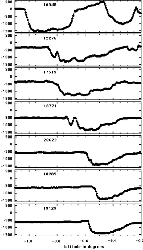
Figure 1. MOLA topography of part of Xanthe Terra extending from 0.5N to 2.5S and from 315.5E to 321.5E, showing the Aromatum Chaos depression and the Ravi Vallis channel system. Each degree of latitude is60 km. Inset shows location of study area. White lines numbered 1 – 7 are locations of the parts of MOLA tracks 16548, 12276, 17319, 18371, 20022, 18285, and 19129, respectively, shown in Figure 6.

water flow speed at each stage. Combining water speeds and depths with corresponding channel widths we obtain volume flow rates. By making assumptions about the sediment-carrying capability of the flood we find an estimate of the minimum duration of the whole water release event and hence of the total volume of water involved and the crustal erosion rate. Our analysis uses a much larger number of channel cross sections than

previous work and so provides a more detailed picture of the history of the formation of Ravi Vallis.

2. Morphology of the Channel System

[5] The floor of Aromatum Chaos rises to about 1 km

below the rim at its eastern end, where it opens out into Ravi Vallis (Figure 1). This opening is the narrowest part of Aromatum Chaos (Figure 2) and forms the highest part of its floor. It is also the highest part of the floor of Ravi Vallis, having an absolute elevation relative to the MOLA datum of about 1200 m. The elevation of the floor of the Vallis decreases from this value to about 1525 m at its connection with Hydraotes Chaos (Figure 1) 205 km to the east.

[6] The mean slope of the floor of Ravi Vallis is found

from the MOLA contours to be0.15. Detailed examina-tion of the contours shows that the slope is close to this average value for the first100 km of the channel, before the bifurcation into northern and southern branches, shal-lows significantly for the next 40 km, and steepens again toward the distal part of Ravi Vallis, reaching a maximum of very close to 1over the last 15 km. We have chosen to focus on the proximal 100 km of the channel, because in this region the slope of the bed is relatively uniform and the cross-sectional profile is less complex, making the analysis and interpretation more reliable. Nevertheless, the floor of the channel is irregular, and consists of a number of subchannels averaging from about 500 to 1000 m wide. The number of these subchannels varies with position from 5 to 13 along the part of the main channel analyzed.

3. Geomorphology of the Channel System

[7] High and low-resolution MOC and THEMIS visible

and infrared images were analyzed to assess the channel floor geomorphology. A number of types of feature were identified that imply that a low-viscosity fluid has flowed through Ravi Vallis. These include teardrop shaped islands, best developed in the more distal parts of the channel system (Figure 3), longitudinal lineations, terraces (Figures 3 and 4), and transverse dunes (Figure 5).

[8] Streamlined islands, common in Martian outflow

channels, are predominantly erosional features indicative of water flow and also of flow direction [Komar, 1983, 1984]. In all cases the orientations of the streamlined islands in Ravi Vallis (Figure 3) are parallel with the general direction of flow implied by the other flow indicators, and their asymmetries are consistent with the sense (i.e., roughly west to east) of the downslope flow.

[9] Longitudinal lineations with ridge-to-ridge spacings

of 250 – 600 m are clearly visible on the floor of Ravi Vallis, showing that deep grooving has occurred [see

Coleman, 2004]. The ridge sides facing away from the

Sun are quite dark (Figure 4), though they do not appear to be in shadow (the solar elevation angle in Figure 4 is 14.3), indicating that, on the 250 – 600 m horizontal scale of the ridges, the bedrock between them has been eroded by no more than perhaps a few tens of meters. Because the widths of the lineations are comparable to the MOLA data point spacing, and the MOLA elevations represent averages over circles 130 m in diameter, we Figure 3. THEMIS-VIS I08290022_B3 showing the

cannot obtain more reliable estimates of the ridge-groove elevation differences from MOLA data.

[10] The transverse dunes visible on the floor of Ravi

Vallis (Figure 5) have orientations consistent with the direction of water flow. However, they would probably show the same patterns if they had been produced by wind reworking of earlier, water-sculpted dunes or of aeolian-deposited sediments emplaced after the flood event.Burr et al. [2002, 2004] used the assumption that water was the causative fluid to explore a potential use of dune

morphol-ogy at Athabasca Vallis in establishing whether flow con-ditions were subcritical or supercritical. However, dunes formed during early, high discharge, supercritical flow can be modified during late stage, waning, subcritical flow and so the implications of their morphology could be ambigu-ous. Therefore we do not use these features in our analysis. [11] The floor of Ravi Vallis also contains two pronounced

patches of chaotic terrain, these being the18 km diameter Iamuna Chaos, located at 0.2S, 319.3E (Figure 2), and the 26.5 km diameter Oxia Chaos, located at 0.2N, 320.0E (U.S. Geological Survey, Gazetteer of Planetary Nomencla-ture, available at http://planetarynames.wr.usgs.gov/, IAU provisional names) (Figures 2 and 3). The presence of these patches of chaotic terrain suggests that local isolated aquifers may have existed in the area prior to the main flood event. Erosion of cryosphere material by the water flood may have reduced the lithostatic load on these local aquifers to the point where they broke through to the surface and added water to the flow coming from Aroma-tum Chaos [Coleman, 2004; Coleman and Dinwiddie, 2005].

[12] There is evidence of terracing of the banks of Ravi

Vallis around the point where Aromatum Chaos and Ravi Vallis join (Figures 2 and 4), and also further down Ravi Vallis (Figures 2 and 3). These terraces provide clear

Figure 4. THEMIS-VIS image V05033001_B3 showing the easternmost part of Aromatum Chaos and the beginning of Ravi Vallis, showing streamlined islands (S), longitudinal lineations (L), and terracing (T). This is the highest part of the floor of Aromatum Chaos. North is to the top. Image width is 17.92 km.

evidence of surface erosion having taken place at a time when fluid was flowing over an area that was significantly wider than the current heavily incised main channel. The most easily identifiable and continuous outermost terrace has a width of25 km and a depth of at most50 m; the topographic slope of the surface defined by its floor is essentially the same as that of the surrounding terrain which, between (1.100S, 317.556E) and (0.661S, 318.409E) (the line marked A-A0 on Figure 2) is tan1(0.0123), i.e., 0.707. A simple interpretation of the morphology is that, some (relatively short) time after the initial water outbreak, either a reduction in volume flux or the onset of bed erosion led to this initial wide channel ceasing to be bankfull, so that the width of the water flood decreased. A longer period of discharge at a relatively constant flux followed, during which the floor of what is now the main channel, typically 15 – 20 km wide, was heavily eroded. Finally, a further reduction in discharge occurred, at which time local

depres-sions in the floor captured much of the water volume, and so the floors of these depressions were deepened, and their walls eroded laterally, to form the subchannels now visible on the floor of the main channel. The presence of these distinct subchannels suggests that the water depth during this period was probably not very much greater than the 50 – 100 m typical depths of the subchannels below the relatively flat, raised areas between them.

4. Estimation of Water Discharge Rate

[13] Measurements were made of the geometries of the

main channel and the subchannels in the proximal 100 km reach of Ravi Vallis using seven MOLA profiles for topographic heights combined with all avail-able MOC and THEMIS images for morphological con-trol. All seven profiles are shown together for comparison in Figure 6, and a representative example, MOLA profile 20022 at longitude 318.312E, is shown in detail in Figure 7, where the individual subchannels on the floor of the main channel are indicated (numbered 1 – 5). Figure 7 also illustrates the basis of the method used to estimate discharges. Horizontal lines were superimposed on the profile of each subchannel in positions cor-responding to hypothetical water surfaces located at 50 m, 100 m and 150 m above the deepest part of the subchannel. Additional horizontal lines were drawn at locations corresponding to any abrupt changes in the slopes of the walls of a subchannel, and also at positions where, if the water level were rising in a channel, it would overspill the lower bank and drain into an adjacent subchannel. If and when this occurred, the two subchan-nels effectively became a single new subchannel with a raised ridge on its floor. Between any two of the horizontal lines, the mean width of the channel was measured and hence the cross-sectional area calculated. For each incremental water depth, D, represented by one of these lines, the mean water flow speed, U, was Figure 6. MOLA data showing geometry and cross

sections of seven channel profiles that were examined at Ravi Vallis. Elevations are relative to Mars datum. Each degree of latitude is60 km.

obtained from the standard Darcy-Weisbach equation for water flow in channels:

U¼½ð8g DsinaÞ=f 1=2

; ð1Þ

where gis the acceleration due to gravity, taken as 3.72 m s2, andais the slope of the channel bed, averaging 0.15 as described in section 2.fis a dimensionless friction factor, values of which are given for a range of bed types on Earth

byBathurst[1993] and are discussed for channels on Mars

byWilson et al.[2004]. An average value offequal to 0.03 was chosen as being relevant to channels 50 – 150 m deep, using the spreadsheet implementing equations (4) to (12) of

Wilson et al.[2004]. Finally, the value ofUdeduced in this way was multiplied by the mean cross-sectional area of the subchannel up to the water depthDto obtain the discharge. The results of this process are given in Table 1 for the 5 subchannels of the typical profile shown in Figure 7. Table 1 also gives the total discharges for the 50 and 150 m water depths. Note that because of changes in cross-sectional shape and the finite depth of the subchannels it is not always easy to obtain flux values at exactly 50 m water depth increments; the values given are therefore for water depths not greater than 50 m and 150 m, respectively. Table 2 summarizes the total water flux values from all 7 MOLA profiles at50 and150 m water depth and gives the average flux for each of these two depths and its standard deviation. The values are (2.3 ± 0.7) 106m3s1and (16 ± 3) 106m3s1, respectively. We stress that these values apply to conditions near the end of the flood event when the subchannel floors had evolved to their shallowest slopes.

[14] For comparison with these values we also calculated

the water flux implied for the early stage flood that formed the terraces on either side of the main channel. As noted earlier,

the relevant parameters areD=50 m anda= 0.71, leading to a mean flow speedU= 25 m s1which, combined with the measured total terrace width of25 km, leads to a flux of30 106m3s1. The likely error in this value, which we estimate at20%, is controlled almost entirely by the uncertainty in the value ofD. This early stage value is essentially double the flux obtained for the late stage discharge if subchannels contained water 150 m deep.

[15] Although we have no way of knowing how much the

discharge varied during the water release event forming Ravi Vallis, we note that, assuming it was fed from an aquifer system to the west via upwelling through the deepening Aromatum Chaos depression, it is likely that the discharge would have initially grown rapidly to a large value and declined thereafter during the erosion of the main channel. A similar pattern of behavior was predicted theo-retically by Manga [2004] for the discharge forming the Athabasca Valles. During the development of Ravi Vallis the slope of the proximal channel floor must have evolved from the initial0.71slope of the prechannel terrain to the Table 1. Discharge Calculations for MOLA Profile 20022 Across Ravi Vallis at Longitude 318.312Ea

Incremental Depth, m

Running Total Depth, m

Average Width of Incremental

Slice, km

Mean Channel Width up to

Running Total Depth, km

Mean Water Speed up to Running Total Depth, m/s

Discharge up to Running Total Depth, m3/s Subchannel 1

20 20 0.59 0.59 7.20 8.54104

30 50 0.99 0.83 11.39 4.73105

50 100 1.28 1.06 16.10 1.70106

50 150 7.80 3.31 19.72 9.78106

Subchannel 2

15 15 0.49 0.49 6.24 4.62104

35 50 1.38 1.12 11.39 6.36105

15 65 1.98 1.31 12.98 1.11106

10 75 2.47 1.47 13.95 1.54106

20 95 5.04 2.22 15.70 3.31106

Subchannel 3

20 20 0.30 0.30 7.20 4.26104

Subchannel 4

25 25 0.59 0.59 8.05 1.19105

15 40 1.38 0.89 10.18 3.62105

10 50 2.37 1.19 11.39 6.75105

Subchannel 5

10 10 0.20 0.20 5.09 1.01104

a

Summary: total discharge (m3/s), water no more than 50 m deep, 1.84106; total discharge (m3/s), water no more than 150 m deep, 1.38107.

Table 2. Total Water Volume Fluxes for Two Water Depths at Ravi Vallis

MOLA Track

Number Longitude,E

Discharge, 106_m3_/s

Water Depth No More Than 50 m

Water Depth No More Than 150 m

16548 317.571 2.64 11.7

12276 317.925 3.16 19.4

17319 317.978 2.85 18.9

18371 318.134 1.45 16.1

20022 318.312 1.84 13.8

18285 318.423 1.33 12.0

19129 318.461 2.52 18.6

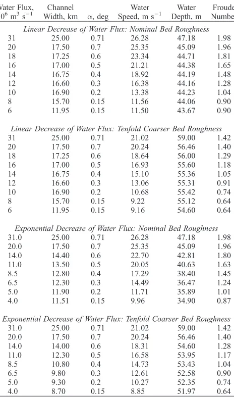
final 0.15 slope observed today. We therefore explore in Table 3 the consequences of two possible histories of the evolution of the proximal part of the Ravi Vallis channel. In both cases the initial flux of3107m3s1is contained in a flood 25 km wide and 50 m deep on the preerosion surface with slope 0. 1. The flux decreases quickly to 2 107m3s1and the flood narrows to the 17.5 km width typical of the eroded channel. Erosion continues with a more slowly declining flux and also a slowly decreasing floor slope (which implies, of course, that the bed erosion rate decreases with distance from the source, a plausible consequence of the increasing sediment load in the water). Two possible patterns of subsequent flux decrease are explored. In the first half of Table 3 the decline is linear with time, and in the second half of Table 3 it is approx-imately exponential. For each row of Table 3, trial and error was used to find combinations of water depth and channel width that are consistent with the pattern of decreasing bed slope and flux values that has been selected and also with

the logical requirement that the occupied width of the channel decreases as the water depth decreases. We do not, however, force the width-depth combinations to be consistent with any actual cross section of the channel.

[16] Table 3 is further subdivided according to the

possi-ble roughness of the channel bed because this can have a bearing on the Froude number,Fr, of the flow, defined by

Fr¼U=ðgDÞ1=2: ð2Þ

If equations (1) and (2) are combined we find

Fr¼½ð8 sinaÞ=f 1=2; ð3Þ

which shows that the Froude number is controlled by the channel floor slope and the bed friction factor. In calculating the flow speeds in Table 3, therefore, we used a formula taken fromWilson et al.[2004] that allows for the influence of both water depth and bed roughness onf:

f ¼8= ð5:62 log₁₀ðD=D84Þ þ4Þ2

h i

; ð4Þ

where 84% of channel bed clasts are smaller thanD84. For

both parts of Table 3 we give the flow conditions corresponding to the nominal value of D84 = 0.164 m

derived byWilson et al.[2004] from rock size distributions obtained from Mars Lander images of the Viking [Golombek

and Rapp, 1997] and Pathfinder [Golombek et al., 2003]

landing sites, and also for a tenfold coarser size distribution withD84= 1.664 m. We chose this value not because there is

reason to think that it is plausible, but because it illustrates that a large change in the friction factor must be made to change the Froude number significantly.

[17] Table 3 shows that whether the water volume flux

decreases linearly or exponentially as the channel is eroded makes only a small difference to the evolution of flow conditions. Using the nominal bed clast size distribution, the Froude number is greater than unity, implying supercritical conditions, during most of the evolution of the channel, whereas using the much coarser bed roughness, conditions are only supercritical for the first half of the life of the modeled flood. Fluid flows in open channels can only become supercritical, i.e., achieve Fr > 1, under certain conditions [Goudie et al., 1994]; specifically, some kind of constricting nozzle, either dictated by preexisting topogra-phy, or developed during sediment deposition from the flowing fluid, is required [Kieffer, 1989]. In this case, the connection between Ravi Vallis and its source in Aromatum Chaos could readily provide such a constriction. However, in water channels on Earth, dynamic interactions between the channel hydraulics and the bed materials, if the latter are sufficiently mobile, appear to evolve in such a way as to prevent the Froude number from exceeding unity for more than short distances or short periods of time [Grant, 1997]. The timescale for these interactions is an important issue, because most of the terrestrial fluvial systems to which these comments apply have had time to reach maturity, whereas water flowed through the Martian outflow channels for relatively short periods, making them much more analogous to the rapidly eroded channels of the Channeled Scablands Table 3. Variations of Water Depth and Water Flow Speed,

Together With Implied Froude Numbers, Required to Accommo-date the Changes of Channel Width, Water Flux, and Bed Slope Suggested for Models of the Evolution of the Ravi Vallis Channel

Water Flux, 106m3s1

Channel

Width, km a, deg

Water Speed, m s1

Water Depth, m

Froude Number

Linear Decrease of Water Flux: Nominal Bed Roughness

31 25.00 0.71 26.28 47.18 1.98

20 17.50 0.7 25.35 45.09 1.96

18 17.25 0.6 23.34 44.71 1.81

16 17.00 0.5 21.21 44.38 1.65

14 16.75 0.4 18.92 44.19 1.48

12 16.60 0.3 16.38 44.16 1.28

10 16.90 0.2 13.38 44.23 1.04

8 15.70 0.15 11.56 44.06 0.90

6 11.95 0.15 11.50 43.67 0.90

Linear Decrease of Water Flux: Tenfold Coarser Bed Roughness

31 25.00 0.71 21.02 59.00 1.42

20 17.50 0.7 20.24 56.46 1.40

18 17.25 0.6 18.64 56.00 1.29

16 17.00 0.5 16.93 55.60 1.18

14 16.75 0.4 15.10 55.36 1.05

12 16.60 0.3 13.06 55.31 0.91

10 16.90 0.2 10.68 55.42 0.74

8 15.70 0.15 9.22 55.12 0.64

6 11.95 0.15 9.16 54.60 0.64

Exponential Decrease of Water Flux: Nominal Bed Roughness

31.0 25.00 0.71 26.28 47.18 1.98

20.0 17.50 0.7 25.35 45.09 1.96

14.0 14.40 0.6 22.70 42.81 1.80

11.0 13.50 0.5 20.05 40.63 1.63

8.5 12.80 0.4 17.29 38.40 1.45

6.5 12.30 0.3 14.49 36.47 1.24

5.0 11.90 0.2 11.71 35.89 1.01

4.0 11.51 0.15 9.96 34.90 0.87

Exponential Decrease of Water Flux: Tenfold Coarser Bed Roughness

31.0 25.00 0.71 21.02 59.00 1.42

20.0 17.50 0.7 20.24 56.46 1.40

14.0 14.00 0.6 18.31 54.60 1.28

11.0 12.30 0.5 16.58 53.95 1.17

8.5 10.80 0.4 14.73 53.43 1.04

6.5 9.80 0.3 12.61 52.58 0.90

5.0 9.30 0.2 10.27 52.35 0.74

[Baker, 1981a], where episodes of supercritical flow appear to have been common.

5. Channel Erosion, Water Volume, and Flood Duration

[18] The total volume of water that must have flowed

through Ravi Vallis can be estimated by measuring the total volume of the valley system and making plausible assump-tions about the sediment-carrying capacity of the water. The cross-sectional area and maximum depth of the valley was determined at five approximately equally spaced locations along its length, chosen to represent both simple and topographically more complex parts of the floor and walls. Where MOLA profiles were oriented roughly normal to the strike of the valley floor these were used directly; elsewhere the gridded MOLA data were used. In each case, the absolute elevations and positions of points on the walls and floor were noted at major slope changes. The position of the prevalley surface was estimated from the trend of the contours near the valley, and the height differences between the present valley topography and the preformation topog-raphy were found by subtraction. Then the cross-sectional areaA and the mean depthD of the resulting topographic profile were obtained numerically from

A¼X

n1

i¼1

0:5DhiþDhjDxij

;

ð5Þ

D¼X

n1

i¼1

0:5 DhiþDhj

Dxij

=XDxij; h

ð6Þ

whereDhiandDhjare successive depth measurements,Dxij

is the horizontal distance betweenDhiandDhj, andnis the

total number of depth measurements, including the first and last value ofDhi= 0 defining the ends of the profile.

[19] Table 4 shows the results. The average of the five

measurements of the cross-sectional area of the Ravi Vallis channel is (2.2 ± 0.9)107m2. By multiplying each area by the fraction of the 205 km length of channel that it represents, the total volume of crustal material eroded to form the channel is found to be 4190 km3. In the same way the overall mean depth of material eroded is found to be 440 m. Models such as those of Clifford[1993] and

Hanna and Phillips[2003] suggest that the cryosphere has a mean porosity of20% down to a depth of1 km. Thus all of the eroded material probably had this porosity, and if this material was ice-saturated, it contained an ice volume of 840 km3, implying an eroded rock volume of3350 km3. However, these values do not represent all of the material that flowed through Ravi Vallis, because the water that eroded the Ravi channel system also removed a large volume of rock and ice from the Aromatum Chaos source depression. In a companion paper (H. J. Leask et al., Formation of Aromatum Chaos, Mars: Morphological de-velopment as a result of volcano-ice interactions, submitted toJournal of Geophysical Research, 2005), we estimate that 3840 km3of rock and 250 km3of ice were removed from Aromatum Chaos, and so the total amounts of material passing through Ravi Vallis were 7190 km3of rock and 1100 km3of ice.

[20] Estimates given byKomar[1980],Smith[1986], and

Costa[1988] suggest that water flowing in channels is able to transport a sediment load of at most40% by volume. If the water flood in Ravi Vallis had this capability, the water volume required to transport 7190 km3of rock would have been (6/4)7190 = 10,785 km3and thus the total volume of water and sediment passing through the valley would have been (10,785 + 7190 =)18,000 km3. From Table 3 the modeled average discharge rates for the flood are 15.0 106m3s1if the flux decrease is linear and 11.5106m3 s1if it is exponential. The implied durations are therefore [(18,000 km3)/(15.0 106 m3 s1) =] 1.2 106 s, or 14 days, in the linear case, and18 days in the exponential case. Given that Table 4 shows the Ravi Vallis channel to be on average a maximum of1000 m deep, this implies an average vertical erosion rate in the channel center of about [(1000 m)/(1.2106s) =]0.83 mm s1, or72 m/d, in the first case, and 94 m/d in the second scenario. These estimates are, of course, strongly dependent on the 40% value assumed for the sediment load of the flood. Table 5 shows corresponding durations and erosion rates for other plausible sediment loads down to 10%; likely values range from2 to8 weeks duration and72 to18 m/d erosion rates in the case of a linear decrease of water flux. The corresponding values are from2.5 to10 weeks duration Table 4. Representative Measurements of Cross-Sectional Area

and Depth of Ravi Vallis Channel

Approximate Longitude of Profile,E

Cross-Sectional Area, 107m2

Maximum Depth of Channel, m

Mean Depth of Channel, m

317.57 2.65 1585 1037

318.00 2.10 848 487

319.00 1.25 550 226

320.00 3.28 1000 502

320.75 2.53 900 402

Table 5. Water Volumes, Flood Durations, and Crust Erosion Rates for Various Assumptions About the Sediment-Carrying Capacity of the Ravi Vallis Flood

Sediment Load Volume, %

Required Volume of Water, km3

Total Volume, Water Plus Sediment, km3

Linear Case Exponential Case

Duration of Flood, days Bed Erosion Rate, m/d Duration of Flood, days Bed Erosion Rate, m/d

40 10,788 17,980 13.9 72 18.1 94

30 16,780 23,973 18.5 54 24.1 70

20 28,768 35,960 27.7 36 36.2 47

and 94 to 23 m/d erosion rates in the case of an exponential decrease. We comment that in our model the exponential decay of the water flux is truncated after the release rate has decreased by about one order of magnitude; if the waning stage extended for a longer time the implied total durations would, of course, increase. In general, the shorter durations and larger erosion rates that we have deduced for Ravi Vallis are comparable to estimates [Baker, 1981a] of the durations and erosion rates ascribed to the Lake Missoula Floods responsible for the erosion of the Channeled Scab-lands in the northwest United States, the features on Earth most commonly likened to the outflow channels on Mars [Baker, 1981b].

6. Discussion

[21] There are a number of ways in which the analysis

described above could be improved. For example, the standard deviations of the fluxes given in Table 2 are based only on the internal scatter of the values listed and do not include a component for errors in measuring the widths of the subchannels. However, given the10 m vertical accu-racy and 300 m horizontal spacing of MOLA data points, measurement errors are estimated to be typically less than 10%, considerable less than the 20 – 30% standard devia-tions of the average fluxes. It is clear that the largest error in the flux estimates is the requirement to make some assump-tion about the depth to which channels and subchannels were filled with water at any one time. However, a more elaborate analysis of the channel system would involve judging the degree of filling of each subchannel relative to an energy surface, i.e., a surface simulating the hypo-thetical continuous water surface within the channel system. Generating such an energy surface within the channel system would be an extremely complex numerical process, even for the well-defined present-day topography of the channel system. We do not feel that this exercise is justified by the relatively small increase in reliability of discharge estimates to be expected from it, as is true elsewhere on Mars [Mitchell et al., 2005], and it would be even more speculative to carry out such modeling for some hypothet-ical intermediate stage in the evolution of the valley. Also, we note thatKleinhans [2005] has recently pointed out an error in the way that Wilson et al. [2004] interpreted the Martian clast size distributions that they used in determining values off, leading to a25% underestimate infand thus a 12% overestimate of U. Given that we have used an average value off, and taking account of the various sources of error just described, this does not significantly change our conclusions.

[22] Our analysis has shown that the morphological

properties of the Ravi channel system can be adequately explained by a single water release event, a conclusion also reached by Coleman [2003, 2004]. This finding can be contrasted with suggestions [Kuzmin et al., 2002;

Rodriguez et al., 2003] that other Martian outflow

chan-nels such as the neighboring Shalbatana Vallis involved multiple water releases over a long, possibly very long, period. If we had found evidence for multiple events at Ravi, this would have supported these contentions. How-ever, the fact that we require only a single flood event at Ravi does not imply that only single events occurred

elsewhere. If the environmental conditions at the times of formation of other outflow channels were similar to those of today, the relative instability of liquid water [Wallace

and Sagan, 1979] makes it unlikely that any of them was

formed by a very large number of very low-discharge events. A detailed physical analysis would be needed to establish the minimum discharge that would lead to liquid water traveling most of the length of any given channel system under a given set of environmental conditions. However, preliminary results [Bargery et al., 2005] based on extensions of the methods of Wallace and Sagan

[1979] suggest that as much a 5 m of depth reduction could have occurred from any given batch of water flowing through the Ravi channel system. This would have a minor impact on our overall discharge estimates for Ravi, but might lead to interesting consequences in any more detailed analysis of the development of the most distal parts of this and other channel systems. These are attractive avenues for future research.

7. Summary

[23] 1. On the basis that Ravi Vallis was formed by a

single water release event through the Aromatum Chaos depression, as evidenced by the presence of lineations, streamlined islands, and chaotic terrain on its floor, we have used the presence of terraces on either side of the main channel system, together with subchannels on its irregular floor, to estimate that water depths during the flood event were probably in the range 50 to 150 m.

[24] 2. These water depths, together with a simple model

of the changing bed slope as erosion took place, lead to estimates (with errors likely to be 20%) of the water volume flux that range from30106m3s1early in the event to less than 10106m3s1in the waning stages.

[25] 3. MOLA data show that the volume of crustal

material eroded from Ravi Vallis and Aromatum Chaos during the flood was8300 km3. Using currently proposed cryosphere models this implies that7200 km3of rock and 1100 km3of ice were removed.

[26] 4. Using a generously high value (40% by volume)

for the sediment-carrying capacity of the flood, the eroded volumes imply that at least 11,000 km3of water passed through the valley system over the course of at least 2 – 3 weeks. Using a more reasonable sediment load of20% the water volume is at least29,000 km3and the duration at least 4 – 5 weeks; with a 10% load the corresponding values are at least65,000 km3and 8 – 10 weeks.

[27] 5. Whatever we assume about the pattern of

devel-opment of the channel system and the roughness of its bed, it is hard to escape the conclusion that the water flow could have been supercritical for as much as the first half of the flood event.

References

Baker, V. R. (1981a), Paleohydraulics and hydrodynamics of Scabland floods, inCatastrophic Flooding: The Origin of the Channeled Scab-land, edited by V. Baker, pp. 255 – 275, Van Nostrand Reinhold, Ho-boken, N. J.

Baker, V. R. (1981b), Large-scale erosional and depositional features of the channeled Scabland, inCatastrophic Flooding: The Origin of the Chan-neled Scabland, edited by V. Baker, pp. 276 – 310, Van Nostrand Rein-hold, Hoboken, N. J.

Bargery, A. S., L. Wilson, and K. L. Mitchell (2005) Modelling catastrophic floods on the surface of Mars,Lunar Planet. Sci.[CD-ROM],XXXVI, Abstract 1961.

Bathurst, J. C. (1993), Flow resistance through the channel network, in Channel Network Hydrology, edited by K. Beven and M. J. Kirkby, pp. 69 – 98, John Wiley, Hoboken, N. J.

Burr, D. M., P. A. Carling, and R. A. Beyer (2002), Investigations into dune features in Athabasca Valles, Mars,Eos. Trans. AGU,83(47), Fall Meet. Suppl., Abstract P71A-0445.

Burr, D. M., P. A. Carling, R. A. Beyer, and N. Lancaster (2004), Diluvial dunes in Athabasca Valles, Mars: Morphology, modelling and implica-tions,Lunar Planet. Sci.[CD-ROM],XXXV, Abstract 1441.

Clifford, S. M. (1993), A model for the hydrological and climatic behavior of water on Mars,J. Geophys. Res.,98, 10,973 – 11,016.

Coleman, N. M. (2002), Aqueous flows formed the outflow channels on Mars,Lunar Planet. Sci.[CD-ROM],XXXIII, Abstract 1059.

Coleman, N. M. (2003), Aqueous flows carved the outflow channels on Mars,J. Geophys. Res.,108(E5), 5039, doi:10.1029/2002JE001940. Coleman, N. M. (2004), Ravi Vallis, Mars-paleoflood origin and genesis of

secondary chaos zones,Lunar Planet. Sci.[CD-ROM],XXXV, Abstract 1299.

Coleman, N. M., and C. L. Dinwiddie (2005), Groundwater depth, cryo-sphere thickness, and crustal heat flux in the epoch of Ravi Vallis, Mars, Lunar Planet. Sci.[CD-ROM],XXXVI, Abstract 2163.

Costa, J. E. (1988), Rheologic, geomorphic, and sedimentologic differentia-tion of water floods, hyperconcentrated flows, and debris flows, inFlood Geomorphology, edited by V. R. Baker et al., pp. 113 – 122, John Wiley, Hoboken, N. J.

Golombek, M., and D. Rapp (1997), Size-frequency distribution of rocks on Mars and Earth analog sites: Implications for future landed missions, J. Geophys. Res.,102(E2), 4117 – 4129.

Golombek, M. P., A. F. C. Haldemann, N. K. Forsberg-Taylor, E. N. DiMaggio, R. D. Schroeder, B. M. Jakosky, M. T. Mellon, and J. R. Matijevik (2003), Rock size-frequency distributions on Mars and impli-cations for Mars Exploration Rover landing safety and operations, J. Geophys. Res.,108(E12), 8086, doi:10.1029/2002JE002035. Goudie, A. S., B. W. Atkinson, K. J. Gregory, I. G. Simmons, D. R.

Stoddart, and D. Sugden (Eds.) (1994),The Encyclopaedic Dictionary of Physical Geography, 611 pp., Blackwell, Malden, Mass.

Grant, G. E. (1997), Critical flow constrains flow hydraulics in mobile-bed streams: A new hypothesis,Water Resour. Res.,33(2), 349 – 358. Hanna, J. C., and R. J. Phillips (2003), A new model of the hydrologic

properties of the Martian crust and implications for the formation of valley networks and outflow channels,Lunar Planet. Sci.[CD-ROM], XXXIV, Abstract 2027.

Hoffman, N. (2000), White Mars: A new model for Mars’ surface and atmosphere based on CO2,Icarus,146, 326 – 342.

Hoffman, N. (2001), Explosive CO2-driven source mechanisms for an

energetic outflow ‘‘jet’’ at Aromatum Chaos, Mars,Lunar Planet. Sci. [CD-ROM],XXXII, Abstract 1257.

Kieffer, S. W. (1989), Geologic nozzles,Rev. Geophys.,27(1), 3 – 38. Kleinhans, M. G. (2005), Flow discharge and sediment transport models for

estimating a minimum timescale of hydrological activity and channel and delta formation on Mars, J. Geophys. Res., E12003, doi:10.1029/ 2005JE002521.

Komar, P. D. (1980), Modes of sediment transport in channelized water flows with ramifications to the erosion of the Martian outflow channels, Icarus,42, 317 – 329.

Komar, P. D. (1983), Shapes of streamlined islands on Earth and Mars: Experiments and analysis of the minimum-drag form,Geology,11, 651 – 654.

Komar, P. D. (1984), The Lemniscate loop—Comparisons with the shapes of streamlined landforms,J. Geol.,92, 133 – 145.

Kuzmin, R. O., R. Greeley, and D. M. Nelson (2002), Mars: The morpho-logical evidence of Late Amazonian water activity in Shalbatana Vallis, Lunar Planet. Sci.[CD-ROM],XXXIII, Abstract 1087.

Leask, H. J. (2005), Volcano-ice interactions and related geomorphology at Mangala Valles and Aromatum Chaos, Mars, M.Ph. thesis, 199 pp., Lan-caster Univ., LanLan-caster, U. K.

Leask, H. J., L. Wilson, and K. L. Mitchell (2004), The formation of Aromatum Chaos and the water discharge rate at Ravi Vallis, Lunar Planet. Sci.[CD-ROM],XXXV, Abstract 1544.

Leverington, D. W. (2004), Volcanic rilles, streamlined islands, and the origin of outflow channels on Mars, J. Geophys. Res., 109(E10), E10011, doi:10.1029/2004JE002311.

Manga, M. (2004), Martian floods at Cerberus Fossae can be produced by groundwater discharge,Geophys. Res. Lett.,31, L02702, doi:10.1029/ 2003GL018958.

Mitchell, K. L., F. Leesch, and L. Wilson (2005), Uncertainties in water discharge rates at the Athasbasca Valles paleochannel system, Mars, Lu-nar Planet. Sci.[CD-ROM],XXXVI, Abstract 1930.

Nelson, D. M., and R. Greeley (1999), Geology of Xanthe Terra outflow channels and the Mars Pathfinder landing site,J. Geophys. Res.,104(E4), 8653 – 8669.

Rodriguez, J. A. P., S. Sasaki, and H. Miyamoto (2003), Nature and hydro-logical relevance of the Shalbatana complex underground cavernous sys-tem,Geophys. Res. Lett.,30(6), 1304, doi:10.1029/2002GL016547. Rotto, S., and K. L. Tanaka (1995), Geologic/geomorphologic map of

the Chryse Planitia region of Mars,U.S. Geol. Surv. Misc. Invest. Map, I-2441.

Scott, D. H., and K. L. Tanaka (1986), Geologic map of the western equa-torial region of Mars,U.S. Geol. Surv. Misc. Invest. Map, I-1802-A. Smith, G. A. (1986), Coarse-grained nonmarine volcaniclastic sediment:

Terminology and depositional process,Geol. Soc. Am. Bull.,97, 1 – 10. Wallace, D., and C. Sagan (1979), Evaporation of ice in planetary

atmo-spheres: Ice-covered rivers on Mars,Icarus,39, 385 – 400.

Wilson, L., G. Ghatan, J. W. Head, and K. L. Mitchell (2004), Mars outflow channels: A reappraisal of the estimation of water flow speeds from water depths, regional slopes and channel floor properties,J. Geophys. Res., 109, E09003, doi:10.1029/2004JE002281.

H. J. Leask and L. Wilson, Planetary Science Research Group, Environmental Science Department, Institute of Environmental and Natural Sciences, Lancaster University, Lancaster LA1 4YQ, UK. (l.wilson@ lancaster.ac.uk)