DEVELOPMENT OF PREDICTIVE SIMULATION MODELS FOR DRUG DISSOLUTION PARAMETERS COMPUTING

International Research Journal of Mathematics, Engineering and IT Vol. 2, Issue 9, Sep 2015 IF- 2.868 ISSN: (2349-0322)

© Associated Asia Research Foundation (AARF)

Website: www.aarf.asiaEmail : [email protected] , [email protected]

DEVELOPMENT OF PREDICTIVE SIMULATION MODELS FOR DRUG

DISSOLUTION PARAMETERS COMPUTING

Dr. H. B. Bhadka

Dean, Faculty of Computer Science, C. U. Shah Univeristy, Wadhwan. Gujarat (India)

ABSTRACT

Over recent years, drug dissolution computing has been the subject of intense and profitable scientific developments. Whenever a new batch profile is developed or produced, it is necessary to ensure that drug dissolution occurs in an appropriate manner. The quantitative analysis of the values obtained in dissolution tests is easier when statistical formulas that express the dissolution results as a function of some of the dosage forms parameters are used. In most of the cases the theoretical concept does not exist and some empirical equations have proved to be more appropriate.

KEYWORDS

Drug Dissolution, Drug release; Drug release models simulation; Parameters Computing.

1. INTRODUCTION

applications. The role of computer based information systems has considerably increased in pharmacy as well as clinical practice in the last decade. However, the use of such systems in dissolution test is still not widespread. Several mathematical systems are commercially available for dissolution parameters calculations. In addition, comprehensive systems customized to specific needs have also been developed. The use of such systems in dissolution parameters calculations, questions regarding the role of structured data versus free text input, standardization of nomenclature, and compatibility with other systems, are hotly debated. This paper has in its scope the above stated considerations in the development of software for dissolution parameters calculations records, which attempts to resolve some of these issues. The model described herein is specifically designed to meet the requirements of the dissolution parameters calculations of a tertiary referral. An additional module has been included to allow modification and update of previously recorded data. A unique number assigned to each has been used as a primary identifier throughout the record.

2. MATERIALS AND METHODS

2.1 Requirements:

The central objective of this initiative is to create a data model capable of accurately representing the calculations for dissolution parameters in a computer-suitable format. The main requirements include that the system should (a) be simple enough to be directly operated by the analytical scientist(s) in analytical research laboratory, (b) can easily run on personal computers, (c) allow comprehensive data entry conforming to accepted procedures which are currently carried out, (d) can generate a printed report, (e) allows modification and update of data, and (f) permit subsequent statistical analysis of records in a tabular format and displays the results of analysis. As dissolution data are to be handled by analytical scientists with minimal previous computer experience, an emphasis is laid on a user-friendly interface.

2.2 Software Construction:

additional module is included to allow modification and update of previously recorded data. Another module is designed for filling test reports on specimens obtained during the procedure, as and when these results became available. A unique identifier assigned to each test record is to be used as a primary identifier throughout the record.

2.3 Data Entry:

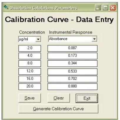
Modules are developed to allow easy user access and facilitate data entry. On completion of one module, automatic transfer to the subsequent module is envisaged. The basic module is structured as a large window, with smaller sub-windows appearing only on demand. The entire software is menu driven, with a simple and consistent hierarchical structure. As far as possible, all fields are structured, with the user allowed to choose one or more options from list of choices. These options included important and/or commonly observed conditions, and are chosen to cover majority of everyday findings after consulting experienced faculty members and reviewing previous records. A standard terminology developed for the structured items based on available literature and general consensus. The fixed choices are displayed either as searchable list boxes, check boxes, or as radio buttons. Free text is allowed in some fields, such as the information beyond the fixed choices available to the user. To allow complete data acquisition in each test, all data fields are

marked mandatory, and the user is not allowed to proceed to a subsequent field without recording data in such fields. (Fig. 1 and 2)

2.4 Debugging and Modification:

After initial development, the software is tested over a four-week period by input of data. An attempt is made to rectify problems faced initially by the users. Opinion is sought from faculty members regarding possible modifications and improvements. Inconsistencies in the programming script, which gave rise to error messages during operation of software, are corrected. Finally the software is put to routine use.

2.5 Software Validation:

the content of information. After entry of data for 60 consecutive test procedures, these details are subjected to statistical analysis to evaluate the robustness of the database component.

2.6 Linearity or calibration curve [6]:

The linearity of an analytical procedure is its ability (within a given range) to obtain test results, which are directly proportional to the concentration (amount) of analyze in the sample. A linear relationship should be evaluated across the range of the analytical procedure. It may be demonstrated directly on the drug substance (by dilution of a standard stock solution) and/or separate weighing of synthetic mixtures of the drug product components, using the proposed procedure. The latter aspect can be studied during investigation of the range.

Linearity should be evaluated by visual inspection of a plot of signals as a function of analyze concentration or content. If there is a linear relationship, test results should be evaluated by appropriate statistical methods, for example, by calculation of a regression line by the method of least squares. In some cases, to obtain linearity between assays and sample concentrations, the test data may need to be subjected to a mathematical transformation prior to the regression analysis. Data from the regression line itself may be helpful to provide mathematical estimates of the degree of linearity. The correlation coefficient, y-intercept, slope of the regression line and residual sum of squares should be submitted for regulatory purpose. A plot of the data should be

included. In addition, an analysis of the deviation of the actual data points from the regression line may also be helpful for evaluating linearity. For the establishment of linearity, a minimum of 5 concentrations is recommended. For the dissolution, concentrations of drug are calculated from the respective calibration curve (Fig. 3).

2.7 Dissolution study [1, 4-5]:

the market. The specifications must be based on the bio-batch dissolution characteristics. If the formulation developed for commercialization differs significantly from the bio-batch, the comparison of the dissolution profiles and the bio-equivalence study between these two formulations is recommended.

The dissolution tests must be undertaken under such conditions as: basket method at 50/100 rpm or paddle method at 50/75/100 rpm. To generate a dissolution profile, at least five sampling points must be obtained of which a minimum of three must correspond to percentage values of dissolved drug lower than 65% (when possible) and the last point must be relative to a sample period of time equal to, at least, the double of the former period of time. For drug products of rapid dissolution,

samples at shorter intervals (5 or 10 minutes) may be necessary. For drug products with highly soluble drugs that present rapid dissolution (cases I and III of BCS), a dissolution test of a single point (60 minutes or less) that proves a dissolution of, at least, 85% is sufficient for batch to batch uniformity control. For drug products containing drugs poorly soluble in water, which dissolve very slowly (case II of BCS), a two points dissolution test, that is, one at 15 minutes and another at 30, 45 or 60 minutes, to ensure 85% of dissolution is recommended (Fig. 4 and 5).

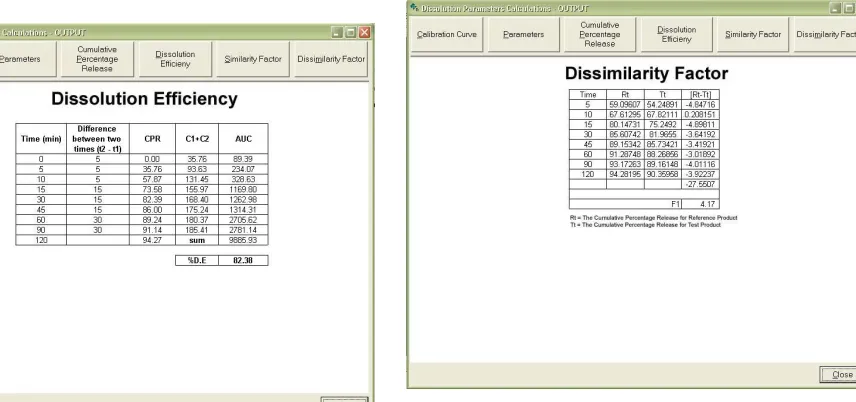
2.8 Dissolution Efficiency [7]:

Khan suggested Dissolution Efficiency (D.E.) as a suitable parameter for the evaluation of in vitro dissolution data. D.E. is defined as the area under dissolution curve up to a certain time „t‟ expressed as percentage of the area of the rectangle described by 100% dissolution in the same time. The D.E. values are calculated from the dissolution data. (Fig. 6)

Dissolution efficiency (D.E.) = ₁₀₀

100 . 0

x y

dt y

t t



2.9 Comparison of dissolution profiles by similarity and dissimilarity factor [2-3, 8-9]:

To avoid the requirement of bioequivalence studies of the immediate release pharmaceutical forms of lower dosage, when several presentations with the same formulation exist, the dissolution profiles must be compared and must be identical among all dosages.

alterations, the comparison of dissolution profiles obtained in identical conditions between the altered formulation and original one, is recommended. In this comparison, the curve is considered as a whole, in addition to each sampling point of the dissolution media, by means of independent model and dependent model methods. Independent model method employing the similarity factor. A simple independent model method employs a difference factor (f1, Fig. 7) and

a similarity factor (f2, Fig. 8) to compare dissolution profiles. Factor f1 calculates the percentage

difference between two the profiles at each sampling point and corresponds to a relative error measure between the profiles:









1 1

1 R R x

f _t t n t t n  





n = number of sampling points

Rt = value dissolved in time t (percentage), obtained with the reference product or with the original formulation (before the alteration)

Tt = percentage value dissolved from the altered formulation, in time t.

Factor f2 corresponds to a similarity measure between the two curves:

               _{ }    



The procedure is described as follows:

 Determine the dissolution profile of products, test and reference, using twelve units of each.

 Calculate factors f1 and f2 using the equations presented previously.

 Criteria for two dissolution profiles to be considered similar.

 The nominal range of f1 and f2 values are 0 to 15 and 50 to 100, respectively.

3. RESULTS

After taking input it display list where user can opt for specific set of computations and can get the results for desired set of computation. The software supplements visualization along with computation. The user can opt for reports to be provided by the software. It generate calibration curve, cumulative percentage release, dissolution efficiency, comparisons of two products through similarity and dissimilarity factors. The software has various modules for input and modification of data, computation of various parameters and visualization with facilities to generate reports of dissolution parameters. The use of interface is designed for work with much ease in respecting. With little practice, scientists soon became adept at entering details correctly and quickly. The slightly increased time of data entry into the computer is more than made up by uniform and complete report generation. A user-friendly software providing computation and visualization parse drug dissolution parameters. The analytical scientists can utilize the software for intensive research as wide variety of parameter computation at simple key stroke.

The computer software currently used has two modules for data input: (a) calibration curve, and (b) cumulative percentage release. The data is linked to a MS-SQL Server having a set of two tables related to (a) calibration curve, and (b) cumulative percentage release and their reports. The two tables are linked to each other using the unique number. Another module deals with screen preview of reports and generation of printed reports.

In the calibration curve module, the number identifies each test record uniquely. The date of

procedure is automatically derived from the system date maintained by the computer clock, but can be changed manually. The user has to enter the number of observations of concentration and instrumental response. After completion of calibration curve test record, the user is transferred directly to the „cumulative percentage release‟ module. The possible locations in the dissolution parameters tree are represented by a cascading hierarchy of tables. An additional table listing the appropriate divisions/segments appears.

On completion of data entry, the user is transferred to the print module, where he can preview the report prior to printing. The printed report contains all the information entered in the database. It also contains a standard set post- procedure instruction for the test, and also has space for signatures for the analytical scientist carrying out the procedure.

printed proforma. However, all agreed that the report and data generated through the software are uniformly complete, and more than made up for the extra time spent. The new report has a uniform and easily understood structure, and is free of any inadvertent omissions.

The database component is evaluated by analyzing 60 consecutive records entered over a 4-month period. Data access and analysis are easily and quickly performed. Data are found to have been completely transferred from data entry screens to the database and no missing values are encountered.

4. DISCUSSION

Structured input and free-text input represent two fundamentally different ways of entering data into a computer. Initial reports of test databases relied heavily on text based tools. Such input facilitates personalized style and flexibility in description of test records, and generates a well readable report. However, free-text input weakens the utility of the database, as it is not suited to subsequent analysis. Structured input and the resulting categorical data offer an important advantage in this regard. Data thus entered is more likely to be complete and is well suited for research and analysis, as well as for the generation of analytical reports and for quality control. It has been estimated that use of computerized test records improves completeness of data entry by more than 50 percent. However, a major trade-off for structure is flexibility. We therefore used a

basic structured data entry protocol, supplemented by use of free text only under special situations. Besides operator related factors, it is related to the amount of free text entered and the number of tables accessed during structured data entry. However, the additional effort is rewarded by a more comprehensive, precise and accurately documented report.

A major feature of the software is the powerful database component. This portion of the software has been built as a set of two interrelated database in MS-SQL Server, which can easily handle large database and also offers a wide range of analytical tools through a versatile query system. We have evaluated the robustness of this module of the software through an analysis of 60 consecutive test records.

ideas and advice. The software has been under routine use, and has performed well in areas of data entry, report generation and data analysis. Successful development and routine application of the database is, however, only a short-term achievement. The system is adaptable and capable of keeping pace with new technological advances.

REFERENCE:

1. “Dissolution testing”, United State Pharmacopoeia, XXIII, NF XVIII, The USP convention, Inc, Rockville, MD, (1995).

2. M. C. Gohel and M. K. Panchal, “Refinement of lower acceptance value of the similarity

factor f2 in comparison of dissolution profile”. Dissolution Technol., vol. 2, pp. 18-22,

2003.

3. M. C. Gohel, K. G. Sarvaiya, N. R. Mehta, C. D. Soni, V. U. Vyas and R. K. Dave, “Assessment of similarity factor using different weighting approaches”. Dissolution Technol., vol. 11, pp. 22-27, 2005.

4. Guidance for industry: Dissolution testing of immediate release solid oral dosage forms. US food and drug administration, Rockville, MD, USA, 1997.

5. Guidance for industry: Immediate release solid oral dosage forms, scale-up and post-approval changes: chemistry, manufacturing and controls, in vitro dissolution testing, and in vivo bioequivalence documentation. US food and drug administration, Rockville, MD, USA, 1995.

6. International conference on harmonisation of technical requirements for registration of pharmaceuticals for human use, ICH harmonised tripartite guideline validation of analytical procedures: Text and methodology Q2 (R1), 2005.

7. K. A. Khan and C. T. Rhodes, “Concept of dissolution efficiency”. J. Pharm. Pharmacol, vol. 27, pp. 48-49, 1975.

8. J. W. Moore and H. H. Flanner, “Mathematical comparison of dissolution profiles”. Pharm. Technol., vol. 20, pp. 64-74, 1996.

Fig. 1 Input form of calibration curve – Data entry

Fig. 2 Input form of Cumulative percentage

release – Data entry

Fig. 3 Output report of calibration curve

Fig. 5 Output report of cumulative percentage release

Fig. 6 Output report of dissolution efficiency

Fig. 7 Output report of similarity factor