The structure of liquid argon as determined by x ray diffraction

(1)

BY X-RAY DIFFRACTION

Thesis by

Bruce Edward Kirstein

In Partial Fulfillment of the Requirements

For the Degree of Doctor of Philosophy

California Institute of Technology Pasadena, California

1972

(2)

i i

(3)

ACKNOWLEDGMEN'rS

I wish to thank Dr. C. J. Pings for his support and the opportunity to study at the California Institute of Technology,

During my graduate studies, I have been the recipient of financial support from the California Institute of

Technology and the National Science Foundation. The funds for this investigation were contributed by the Air Force Office of Scientific Research, Directorate

of Chemical Sciences,

This investigation would not have been possible

without the help of the people in the Chemical Engineering shop, George Griffith, Chic Nakawatase, Bill Schuelke, John Yehle, Ray Reed, and also Hollis Reamer who supplied invaluable aid in the laboratory.

The data handling and subsequent numerical studies using the computing facilities were made possible with the help of Kikuko Matsumoto, Martha Lamson, Edith Huang, Joe Dailey and the entire operating crew, in particular the night crew, Jorge Gonzalez and Mike Martinov.

(4)

iv

(5)

ABSTRACT

X-ray diffraction measurements and subsequent data analyses have been carried out on liquid argon at five states in the density range of 0.91 to 1.135 gm/cc and temperature range of 127 to 14J°K. Duplicate measure-ments were made on all states. These data yielded radial distribution and direct correlation functions which were then used to compute the pair potential using the Percus-Yevick equation. The potential minima are in the range of -105 to -120°K and appear to substan-tiate current theoretical estimates of the effective

pair potential in the presence of a weak three-body force. The data analysis procedure used was new and does not distinguish between the coherent and incoherent absorption factors for the cell scattering which were essentially equal. With this simplification, the argon scattering estimate was compared to the gas scattering estimate on the laboratory frame of reference and the two estimates coincided, indicating the data normalized. The argon scattering on the laboratory frame of reference was examined for the existence of the peaks in the struc-ture factor and the existence of an observable third peak was considered doubtful.

(6)

Vi

radial distribution function, uncertainties in the low angle data relative to errors in the direct correlation function and the distortion phenomenon are presented.

The distortion phenomenon for this experiment explains why the Mikolaj-Pings argon data yielded pair potential well depths from the Percus-Yevick equation that were too shallow and an apparent slope with respect to density that was too steep compared to theoretical estimates.

(7)

TABLE

OF

CONTENTS

(9)

r'NDEX FOR FIGURES

page 1. Argon pressure-density phase diagram 52

showing locations of experimental states 2. Example of raw data, 2/23/71

J. Example of raw data, 7/28/71 4. Example of raw data, 12/15/71

5. Example of argon spectrum, 11/J0/71 6. Example of argon spectrum, 12/15/71

53 54 55 56 57 7. Example of data analysis, 11/J0/71 58

(7.A through 7.M)

8. Example of data analysis, 12/21/71 71 (8.A through 8.M)

9. Computed Percus-Yevick well depth for 84 for each experiment

10. Main peak height of i(s) for each 85 experiment

11. Main peak height of g(r) for each 86 experiment

12. Main peak height of c(r) for each 87 experiment

13. Width of main peak of i(s) at i(s)

=

O 88 for each experiment

14. Numerical experiment on effects of 89 distortion (14.A through 14.G)

15. Numerical experiment on the subsidiary 96 peak in g(r) (15.A through 15.E)

16. Numerical experiment on effect of low 101 angle smoothing (16.A through 16.G)

(10)

x

INDEX FOR FIGURES

page 18. Numerical experiment on g(O)>O 112

(18.A t hrough 18.D)

19. Comparison of computed Percus-Yevick 116 well depths with theoretical result

of Rowlinson

A.1 Dual Filter Spectra 300

B.1 Atomi c Scattering Factors for Beryllium 309 B.2 Atomic Scattering Factors for Argon 310 C.1 Cross Section of Cell Relative to X-ray 321

Beam Illustrating Dimensions Required to Compute Absorption Factors

D.1 Results of Numerical Test of Spline 363 Smoothing Computer Program

D.2 Example of Spline Smoothing Applied to 364 NMR Data

F.1 Results of Example Calculation, Fourier 375 Transform (F.1 through F,2)

G.1 Illustration of Scattering at 8₀ 391 G.2 Illustration of Divergent Scattering at 392

90

G.3 Illustration of Divergent Scattering at 393

8

0 Viewed from X-ray Source

(11)

INDEX FOR TABLES

page 1. Cross Reference: Date of Experiment - 117

Thermodynamic State of Argon

2. Cell Subtraction Factors, F (see Eq. 15), 118 and Smoothing Input Information

J.

Thermodynamic Data for Argon 120

4. Intensity Measurements (total counts) 121 for Each Experiment (4.A through 4.K)

5. Data Analysis for Each Experiment 154 (5.A through 5.K)

6. Data Summary: Main Peak Height of g(r), 220 c(r), PY Well Depth, Main Peak Height of

i(s) and Width at i(s)

=

0

7. Numerical Experiment: Distortion (7.A through 7.D)

222

8. Summary of Effect of Distortion on PY 246 Well Depth

9.

Numerical Experiment: Subsidiary Peak 247 in g(r)

10. Numerical Experiment: Low Angle Smoothing (10.A through 10.B) 11. Numerical Experiment: Truncation

(11.A through 11.B)

12. Numerical Experiment: g(O)~

+J

(12.A through 12.B)

1J. Numerical Experiment: Absorption Factors

253

265

277

289

A.1 Dual Filters: Thickness-Transmission 301 A.2 Dual Filter Spectra

B.1 Interval Identification for Spline Interpolation of Atomic Scattering Factors

J02

(12)

xii

INDEX FOR TABLES

page

B.2 Cubic Spline Interpolating Coefficients 312 for Beryllium Scattering Factors

B.3 Cubic Spline Interpolating Coefficients 313 for Argon Scattering Factors

B.4 Scattering Factors for Data Analysis 314

C.1 Absorption Factors for Each Experiment 322 (through C.12)

G.1 Maximum Divergence for Sample-Detector 395 Distance of 6-J/4 Inches and Sample

Length of J/8 Inch

G.2 Results of Distortion Correction for 396 Numerical Example

(13)

I. INTRODUCTION

Information about the structure of an ensemble of

spherically symmetric atoms is needed to test statistical

mechanical theories of fluids. These theories attempt

to describe the physical properties of such systems based

on the configurational energy of its particles. Efforts

have been made in the past to determine the structure of

1,2 J-8

argon and other fluids using x-ray or neutron

dif-fraction data. A summarization of the most recent results

may be found in Simple Dense Fluids, edited by Frisch

and Salsburg.9

Since the computations required in statistical

mechanics are not simple exercises, and since the

.dif-fraction experiments to determine the structure present

many problems in technique and numerical analysis which

drastically affect the final result, i t is then indeed

difficult to ascertain if differences in theory and

experiment are due to technique, poor theory or both.

Reasonable agreement between experiment and theory in

the past has not been obtained.

The general subject of experimental technique

rela-tive to the structure determination of simple fluids

by x-ray diffraction has been reviewed recently by Pings.10

The scattering of radiation by matter will involve

(14)

2

of radiation is of the order of the interatomic distance.

The scattering from each atom will constructively or

destructively interfere with the scattering from other

atoms depending upon their relative locations. The

distribution of positions of interest in fluid argon or

for an ensemble of spherically symmetric scatterers is

called the radial distribution function, written

hence-forth as g(r). This function is also called the pair

distribution function and is the relative probability

of finding an atom at a distance r in a differential

volume element if there is an atom at the origin,

nor-malized to unity at large r. Written in equation form,

g(r) = p(r)/p, where

p

is the bulk density.

The coherently scattered radiation, I(s), in an

x-ray experiment for such a system of atoms is related

to g(r) by1ll-lJ

i ( s)

and

=

I(s) -1

=

4:PJ =lg(r)-1]sin(sr)dr f 2(s)

0

s

=

where s is termed the scattering parameter, uniquely

determined by one-half the scattering angle, 9, and

( 1 )

(15)

the wavelength of the radiation,

A,

l(s) ls the

struc-ture factor and f 2 (s) ls the atomic scattering factor.

Coherently scattered radiation means there ls no

wave-length change in the scattering process as there ls in

Compton scatterlng.14

The integral equation for l(s) and hence I(s) may

be formally inverted to yield g(r) as a function of i(s):

g(r)-1

=

(277'2pr)-lf :l(s)sin(sr)ds

. 0

( 3)

Another quantity of interest in statistical

mechan-ics is the direct correlation function, c(r), introduced

by Ornstein and Zernlke1

5

in 1914:

c(l'j_ 2 )

=

h(r

12)-p

f

:<I'i

3)h(r23JdrJ 0

( 4)

where h(r) ls g(r)-1. The definition of c(r) ls basically

mathematical and the function lacks an obvious physical

interpretation such as that assigned to g(r). Goldstein16

has subsequently shown that c(r) can be rigorously

com-puted from diffraction data by the following expression:

c( r)

= (

277'2Pr

r

1

1:1 (

s) 11

+1(

s)

r

sin( sr )ds 0

( 5)

(16)

4

as PY theory, is of current interest and relates the

pair potential, u(r), to the two quantities g(r) and

c(r) by the following approximation1

u(r)

=

kT*ln[l-c(r)/g(r)] ( 6)

where T is the absolute temperature and k is the Boltzmann

constant. The above approximation may be obtained by

examining the density expansion of g(r) and c(r) in

terms of graph theory

18

assuming that the configurational

energy of the system may be obtained by considering only

pairwise interactions. Essentially, terms greater than

order two in density are neglected and two graphs in

the second order term of c(r) which lack a Mayer f 1

2 bond are neglected. However, in the limit of zero

density the approximation becomes exact.

It is anticipated that the pair potential would

be state independent as predicted by PY theory. However,

if the theory predicts a state dependence of the potential,

then the conclusion could be drawn that the components

of the system do not interact strictly pairwise, the

theory is incorrect in neglecting some terms, or the

experiment itself including the numerical analysis is

not correct.

It has, therefore, been the attempt of this thesis

(17)

analysis relative to an x-ray diffraction experiment to determine g(r) and c(r) for a simple fluid. The net result has been better control of the experiment. Also a relatively new approach to the numerical analysis

involving calculation of absorption corrections, smoothing of data, distortion corrections and Fourier transforming has been developed.

There is now substantial evidence that the config-urational energy of a dense fluid will have to include more than just two-body interactions.19- 32 Then the

PY theory as previously stated and other theories are not expected to predict a state independent pair potential for this reason, and the interest now is how the potential varies as a function of density.

Recent efforts by some investigators33-3

6

have involved computing an effective pair potential in the presence of a weak three-body force. There is more than one such effective potential since the examination of different properties leads to different effective poten-tials. 34 The relevant effective potential then is the one that yields the correct radial distribution and

(18)

6

but the result obtained will then be an estimate of the effective pair potential. A comparison between experi-ment and an assumed configurational energy which includes a weak three-body force may then be made through this

computat ional trick involving an effective pair potential. The work of Rowlinson,35,36 et al, computes the

effective pair potential for argon that yields the cor-rect radial distribution function from the configurational energy through the

p2

term of a system that includes a weak t hree-body force. These results also provide the non-addi tive contributions to the fourth virial coeffi-cient for the same force, The calculation requires that a zero density value for the pair potential be introduced since the form of the equation yields the result (u*-u)/kT where u* is the effective pair potential and u is the

zero density pair potential. Rowlinson uses the zero density pair potential of Barker and Pompe 19 which has a minimum of -148°K to plot the actual minimum of u*/k. There are other estimates of the zero density potential and the more recent estimates have minimum values ranging from that of Barker and Pompe's up to approximately

-140°K,37

(19)

an effective minimum of -125°K at one gm/cc for argon. There is a slight upward curvature of u*/k with increas-ing density reflectincreas-ing the

p2

contribution.

The data of Mikolaj and Pings38 are compared to this effective potential and i t is observed that there is a large discrepancy, the experimental minimum of the poten-tial being much too shallow and having a positive slope with respect to density tentatively observed as being slightly too large. These differences to this date have not been explained and i t is difficult to believe that the difference is due to non-additive effects. Other investigators have made the same observations. 1 9,39,

4

o

The result of this thesis, which describes diffrac-tion measurements and subsequent data analysis on five thermodynamic states of argon in the liquid region, as indicated in Figure 1. and Table 1., essentially confirms the stated work of Rowlinson and also explains why the Mikolaj-Pings data behave as they do.

The most important experimental phenomenon which was neglected in the past is that of a distortion effect resulting from an x-ray detector accepting a finite

(20)

8

and always being nonzero for finite densities.

Error bands for the data in this thesis were not calculated because of the uncertainty of the validity of such a calculation. Each thermodynamic state was measured at least twice to give some measure of repro-ducibility. Information in t he form of numerical experi-ments is now presented that indicates that error bands previously estimated do not take into account the observed reproducibility.1•2 The major effect observed is uncer-tainty in the low angle data and hence affects c(r) for thermodynamic states wi t.h relatively small isothermal compressibilities.

.

2 4 41-45

The phenomenon of the subsidiary peak ' ' in

g(r) was observed, but only sometimes. Data are pre-sented which show that a perturbation in the smoothing of the raw data within reasonable error bands may cause such subsidiary peak to appear or disappear.

The data analysis to be presented makes use of the behavior of g(r) in the region of

0$r~JR.

Data are some-times presented in the form r [g(r)-1] and this behavior is then masked. The desired result now appears to have g(0)-1 be close to -1. This involves evaluating the sine transform of si(s) for r=O which is1

(21)

This is essentially the normalization suggested by

Krogh-Moe. 46 If positive g(0)-1 values are allowed, the

Percus-Yevick well depths will decrease about 5°K for

every

+J

units of g(0)-1 as indicated by transforming

actual experimental results.

The truncation of the structure factor in this work involved estimating what could be observed from the data

on the laboratory frame of reference. Essentially no

third peak in i(s) was observed at pressures of 19 to

J?

atmospheres at 127°K. However, a third peak could barely

be inferred at 54 atmospheres and 127°K. As the pressure

decreases, the peaks in i(s) are expected to decrease due

to a reduction in packing and hence the third peak at

lower pressures was not included. It was anticipated that

any attempt to include the third peak would result in an

incorrect period of oscillation40 and peak height, and

since i(s) must be multiplied by s for the Fourier

trans-form, the resulting error would be unpredictable. The

data at 54 atmospheres were transformed for both g(r) and

c(r) with and without the third peak in i(s) and the

dif-ferences indicated a 2°K change in the PY well depth.

Three valleys in i(s) were always observed and i(s) was

truncated at its zero in the region of s

~

5

~-l.

Numerical experiments are presented in table and

plotted form to indicate the reasoning for the various

(22)

10

II. APPARATUS

The equipment used to confine a sample of fluid argon

(99,996%

pure) was essentially the same as that of Mikolaj1 and Smelser. 2 Changes were made only to the peripheral support equipment. The temperature measuring and control system used was a modification of a method described by Daneman47 and also previously used by wu48 in this laboratory. The pressure measurement and control were obtained by an oil-piston system also used by Wu. Both the temperature control and pressure measuring techniques mentioned above were new to the x-ray experi-ment and were primarily intended for use in the study of the index of refraction of argon in the critical region.48 For the data obtained in this thesis, temperature was

controlled to within +0.002 degrees Kelvin and pressure was controlled to within ~0.2 psia.

(23)

These improved vacuums were the result of using SARAN WRAP® to cover the x-ray slot in the cryostat. Pre-viously Mylar® had been used. 1 •2

The sample cell was constructed of sintered beryllium 2

and described by Smelser. Cell dimensions of importance

for calculating absorption corrections are the inside and outside diameter previously quoted at 0.035 and 0.070 inch respectively. These dimensions were

reason-ably verified by observing the apparent size of the cell with x-rays and knowing the distance of the detector and cell from the x-ray source.

The goniometer and cell were aligned essentially

as described by Smelser.2 The only modification that occurred was the alignment of the 0.005 inch receiving sellers. The actual alignment of the detector required

the use of a LiF single crystal, incident slit and a

very narrow receiving slit. Once alignment was obtained,

the receiving slit was removed and the receiving sellers were mounted. The entire receiving assembly was then

"rocked" while looking at a strong Bragg peak to maximize

the intensity. This operation set the receiving assembly platform parallel to the scattered rays coming from the goniometer axis. Upon removing the receiving sellers and

mounting the receiving slit again, the alignment was

(24)

12

changed by the "rocking" of the receiving assembly.

Therefore the receiving slit had to be realigned. After

this second alignment, the receiving sellers still

re-quired a further fine adjustment to insure that they were

looking at the goniometer axis. It should be noted that

the sellers were 0.005 by 1.25 inches and an error

involving the front or rear being 0.001 inch too high or

low would foreshorten the view of the region of the

goniometer axis. The receiving sellers were then adjusted

by inserting a metal shim under the front or rear as was

needed. This final adjustment did not upset the

align-ment as determined by the receiving slit.

The pertinent dimensions of the x-ray path were as

follows. The beryllium cell was 18 cm from the x-ray

tube target. The incident slit was a 1/6 degree

diver-gence slit, ·0.006 inch, located 8 cm from the x-ray tube

target. Vertical incident sellers, 0.01 by 1.25 inches,

were mounted between the x-ray tube and incident slit.

The take-off angle from the x-ray tube target was

5!

degrees. The sample-detector distance, with the rear of

the receiving sellers defining the detector face, was

17.1 cm.

The x-ray source was a Norelco® full wave generator

and a Standard Focus X-ray Tube, molybdenum target, model

(25)

state high voltage rectifiers were used instead of the

vacuum tube type and this appeared to improve stability.

The x-ray detection and recording system was

com-pletely changed from past experiments. 1 •2 An Amperex®

XP1010 photomultiplier with a

Horiba~

4HG2 sodium iodide

crystal formed the x-ray detector. The dynode chain

was constructed with 150,000 ohm resistors instead of

the normal 470,000 ohm. This decreased resistance drew

approximately ~ ma from a Hewlett Packard Model 5551A

high voltage power supply operated at +1200 volts.

Detector resolutions on the order of 28% were consistently

obtained with this improved system.

The increased dynode current greatly decreased the

gain shift phenomenon. The gain shift in a photomultiplier

is caused by the current due to the electron transfer

between dynodes becoming an appreciable fraction of the

total current through the entire dynode chain and

upset-ting the voltages between the dynodes. This effect will

cause a decrease in the gain of a system.

Data recording and goniometer positioning was

obtained through the use of a Canberra Industries DATANIM®

system and a Cipher Data Products Model ?OH magnetic tape

recorder. This system was a ten instruction programmable

computer which allowed complete automation of the

goni-ometer positioning, x-ray counting and recording, and

(26)

14

III. DATA ANALYSIS

A. Introduction to Data Analysis

The objective of this x-ray diffraction experiment

on argon was to determine the quantity called the

struc-ture factor, i(s), as defined in Eq. (1). The structure

factor had to be determined over the range where i t was

nonzero so that i t could be Fourier transformed for the

radial distribution and direct correlation functions as

defined in Eqs.

(J)

and

(5).

The data analysis procedure

used here has produced some insight as to the sensitivity

of the above auantities to the various techniques used

or decisions that had to be made.

Invariably, the procedure to determine the structure

factor in this type of experiment, and hence g(r) and

c(r), is a technique. A technique in this context is

defined to be a procedure that requires the user to make

a decision or decisions that may be somewhat subjective.

The numerical techniques used in this thesis differ from

those used previously. 112 The previous techniques,

though quite correct on paper, did not lend themselves

to clearly defined procedures.

The data analysis to be described is based on a

monochromatic x-ray source obtained through the use of

dual filters which are described in Appendix A.

(27)

performed using actual data to render justification of the decisions made, These numerical experiments are

described in Section V. and are referred to where neces-sary. The numerical experiments are the following:

A. Effect of Distortion on g(r) and c(r).

B. The Subsidiary Peak Phenomenon.

c.

Effect of Uncertainties in Smoothing the Low

Angle Data on g(r) and c(r).

D. Truncation, The Existence of a Third Peak in

i(s) at Various Pressures and the Effect of

Neglecting It.

E. Effect on g(r) and c(r) when g(O) is

Signifi-cantly Different from Zero.

F. Effect on g(r) and c(r) of Using Post- vs.

Pre-cell Alignment for Computation of

Absorption Factors.

Because of the interference of the main beam, the auantity I(s) could only be determined with the equipment

used in this thesis down to an s value of about 0.4

R-

1 , which was about

2

t

degrees in 20 space. The s

=

0 value of i(s) is known to be:

4

9

i(O)

= PkTK - 1

( 8 )

where K is the isothermal compressibility. The usual

practice, and used here, is to interpolate over the

(28)

16

where a and b are constants to be determined from the

data.

( 9 )

At high values of s the x-ray scattering for argon is expected to be the same as the gas scattering which is just an ensemble of non-interacting atoms. Note that scattering at high s values reflects scattering from two

centers that are relatively close, namely intra-atomic electrons. Deviations from the independent atom

scatter-ing or gas scattering reflects structure or preferred positions which occur at lower values of the scattering

parameter, s.

Therefore, experimental data were obtained in this work to sufficiently large values of s so that the com-parison to the gas scattering could be made and I(s) could then be scaled to the same frame of reference as

f 2 (s).

(29)

B. General Data Analysis

The scattered radiation from a cell and argon sample as the result of being irradiated by a monochro-matic beam of x-rays may be written as:

where 28 is the scattering angle, Na and Nc are normali-zation constants, 1~(28) and 1;(28) are the coherent and incoherent (Compton14 ) scattering from the argon sample,

A~(28)

and A;(28) are the coherent and incoherent

absorp-c i

tion factors for the argon, Ic(28) and Ic(26) are the coherent and incoherent scattering from the cell, A~(26)

i

and Ac(28) are the coherent and incoherent absorption factors for the cell, and P(26) is the polarization factor given byi14

( 11 )

The quantity to be determined from data in Eq. (10) ls 1~(26) which is I(s) in Eq. (1).

(30)

18

experiment. The empty cell scattering may be written

ass

where the subscript ec denotes empty cell.

Note that i t appears that the distinction must be

made between coherent and incoherent radiation because

of the absorption factors which are wavelength dependent,

I

14

with the incoherent wavelength,

X,

given by1

( 13)

where

A

is the coherent wavelength. However, upon

calcu-lating absorption factors as described in Appendix D for

this particular experiment for Mo

Ka

radiation, the fact

emerged that for the cell, the difference between the

incoherent and coherent absorption factors, with or

with-out the sample present, was small and on the order of

0.002 at 60°

28.

This fact may also be observed in a

previous thesis.2

At this point in the data analysis the distinction

between the coherent and incoherent absorption factors

for the cell was ignored. Both types of absorption

(31)

( I

the difference was small. This assumption that the

coherent and incoherent absorption factors for the cell

were eoual is the major difference in the data analysis

1 2

procedure from the previous two theses. ' Note that

this assumption was not applied to the sample.

Therefore, letting

A~c(28)

=

A~c(28),

Eq. (12)

becomes:

( 14)

*

where Ic(28) is the total scattered radiation from the

cell. Also, letting Ac(28) i

=

Ac(28), c

Eq.

(10) becomes:

( 15)

Therefore, to subtract the cell scattering from the

cell plus sample scattering, the empty cell data could be

c c

divided by Aec(28) and multiplied by Ac(28) and the

subtraction carried out. This was not done.

The subtraction procedure above is correct only if

the same amount of rad.iation was delivered to the two

separate expe~iments and the cell position was the same

(32)

20

cell did move slightly during t he experiments descrlbed here.

In order to observe and minimi ze t he effect of the

intensity drift, the entire 28 space under study was scanned many times, with each complete scan requiring

one to two hours. Then at the end of the experiment , the scans were simply added together for each 28, thus mimicking a multichannel analyzer. This technique had the advantage that the maximum drift in any single scan would be that which had occurred over the time period

of that scan.

In order to scale the empty cell data to the cell plus sample data on an intensity basis, the drift in the summed counts for each scan was studied. The advantage of using the summed counts for a scan verses a single Bragg peak or flat region in the scan was that the

summed counts yielded a much larger number and in terms of statistics a much smaller drift could be observed.

(33)

The actual cell movement observed over the time period of an experiment was usually less than 0.001

inch as indicated by alignment checks before and after the experiment. However, with the cell moving, note that the number of scattering centers in the x-ray beam would change and an apparent intensity drift would then be observed. Also with cell movement, the alignment would change and thus affect the absorpti on factors.

To ascertain the effect on the data due to a change in absorption factors because of cell movement, the

absorption factors were computed from the cell positions at the beginning and end of one experiment and the data

0

subsequently analyzed, The effect was approximately 2 K on the PY well depth and considered negligible.

The apparent change in intensity as indicated by the summed counts for a scan could not be definitely assigned to either incident intensity drift or cell

movement. Since the relative change was never more than one to two per cent, and since the empty cell and cell plus argon were irradiated for the same lengths of count time, and since the total time for the entire experiment was on the order of 24 hours, the empty cell data were usually subtracted off with a scale factor, F, of about unity. The actual F factors used are presented in

(34)

22

Hence, the argon scattering alone may be written

as:

where Ia(28) is the total argon intensity. The argon

intensity above is also the first term on the right hand

side of Eq. (10).

At this point in the data analysis i t was necessary

to smooth the argon scattering curve and then correct i t

for distortion. The distortion correction technique

requires derivative estimates which were obtained from

the smoothed line estimate.

The smoothing technique used is an adaption of the

cubic spline interpolation method and this is the

first time i t has been applied to this type of x-ray data.

This smoothing technique fits piecewise cubics to a set

of data, but now using least squares criterion and

demanding continuity in the function and first

deriva-tive over the entire smoothing range. The derivation

of this smoothing technique is presented in Appendix D.

However, like any technique, the user must make

some decisions relative to its use. In spline smoothing

the user must know or estimate the values of the function

(35)

For the data analysis here, the value of the func-ti on at 28

=

0 simply had to be guessed because of dis-tortion effects, but the derivative was zero because of symmetry. At t he upper value of the independent vari-able the argon scattering curve behaved like the gas or independent atom scattering of x-rays, namely:

(17)

where the independent variable is now changed to s as defined by Eq. (2), noting that Mo

Ka

radiation was used. All the quantities on the right hand side of Eq.

(17)

were known in a particular experiment except the normali-zation constant, Na. Ia(s) was easily estimated from the data at large values of s since the curve was rela-tively flat. rherefore Na was determined and a derivative estimate was computed for input to the smoothing routine.

(36)

24

all degrees of freedom and decrease the variance to zero.

The input used to smooth the data for each experiment

described here is presented in Table 2.

After the data were smoothed, t hey were corrected for distortion, The distortion effect arose from the

fact that the detector accepted a finite angular spread of scatt ered radiation, The description of the distor-tion correcdistor-tion that applied to this experiment is pre-sented in Appendix G.

After the data had been smoothed and corrected for distortion, the structure factor, i(s) could then be

determined, At this point the scattering data were still of the forms

( 18)

Here a decision had to be made and that was the point at which i(s) went to zero, This point is referred to as the truncation point. This decision was made by visual examination of the data. The truncation point that was used for all experimental states was in the region of

5

<

s

<

5, 5 R-1

which roughly corresponded to

2~ oscillations of i(s) or the fifth zero in i(s). Suppose that the truncation point chosen was s

0 ,

(37)

Ia(s), was described by the gas scattering at that point

which then determined the normalization constant:

This normalization constant may be close to the one used

in the smoothing step but not necessarily the same.

With the value of Na determined, I~(s) could then be

determined from the data:

i

where Ia(s) is the theoretical value of the incoherent

atomic scattering. The structure factor, i(s) was then

computed using Eq. (1). The scattering factors used in

this thesis are presented in Appendix B.

At this point a consistency check could be made

on the choice of the truncation limit or actually Na.

The r

=

O value of g(r)-1 is computed by:

g(0)-1=(277"2p)-l1•: 2

1(s)ds

0

( 21)

Theoretically g(O)

=

0 so that the value of the integral

should be close to

-21T2p,

This is essentially the

(38)

26

Note that the truncation procedure used chopped off a third peak in I(s) because i t was not visible. Since the i(s) curves included two positive peaks and three negative peaks, i t was anticipated that g(0)-1 would be biased in the negative direction, A rule of thumb

criterion in computing i(s) was to demand that the value of g(0)-1 be not greater than -1 or smaller than

-J

and preferably between

-J

and -2. Therefore a trial and error procedure developed in choosing the truncation point.

Much discussion has ensued about the observability of the third positive peak in i(s) and its effect on the results. Clearly the exclusion or inclusion of this peak will affect the g(O) calculation. Numerical experiments on both of these topics are presented in Section V.

The technique used to Fourier transform the struc-ture factor is that of integrating an analytic approxi-mation. The structure factor was obtained as a set of smoothed points. These points were interpolated using the cubic spline interpolation presented in Appendix E. Appendix F indicates the algebra necessary to use the piecewise cubics in a Fourier transform.

(39)

1. Compute absorption factors for the observed alignment of the cell in the x-ray beam. 2. Subtract the cell data from the cell plus

argon data to obtain the argon scattering.

J.

Smooth the argon scattering which involves

a guess of the normalization constant.

4.

Correct the argon data for distortion

effects.

5.

Guess a truncation point on the argon scattering curve and compute i(s).

6.

Compute g(O), if this value is not acceptable, repeat step

5.

(40)

28

IV. DATA PRESENTATION

&

DISCUSSION

Table 1. is a cross reference between the date of the experiment and the thermodynamic state. Each experi-ment is uniquely identified by a date because each

thermodynamic state was studied at least twice. Figure 1. is a pressure-density phase diagram for argon locating the thermodynamic states that were studied. Table

J.

presents the i(O) values obtained from Levelt51 and Itterbeck. 52

are1

The data presented for each of eleven experiments

1. Absorption factors, Tables C.1 through c.12 in Appendix

c.

2. Intensity measurements after summation of the scans and dual filter subtraction, and the argon spectrum, Tables 4.A through 4.K. (The *by a datum indicates that i t was

deleted in the smoothing step.)

J.

Smoothed argon spectrum before and after the distortion correction, i(s), g(r),

c(r) and PY u(r)/k, Tables 5.A through 5.K. Examples of the raw data on the laboratory frame of reference for the experiments of 2/23/71, 7/28/71

and 12/15/71 are presented in Figures 2. through

4.

These data are the starting point for the data analysis to

obtain g(r) and c(r). Observe the low angle region in these Figures and note that the empty cell scattering should go to zero at 28

=

0 because beryllium is

(41)

this appears to be t he case but not for the data of 7/28/71 and 12/15/71. The data in the last two Figures show an enounter of the x-ray main beam. This occurred because the receiving slit on the detector was opened up to insure observation of all of the cell at high

values of 28 and hence prevent any rotation of the data. 1

The upswing of the low angle cell plus sample data of 2/23/71 is due to the isothermal compressibility of argon. The raw data from all experiments were plotted in this manner and the main beam encounter was noted.

The subtraction procedure to obtain the argon

scattering did not necessarily recover the argon scatter-ing at low angles when the main beam was encountered as i t might be assumed. Therefore the datum that indicated i t was contaminated by the main beam was usually deleted.

Also note in Figures 2. through

4.

in the region of 20° 28 that the beryllium peaks are very large relative to the argon scattering. This is the region of the second peak of i(s) for argon.

(42)

JO

of the data. One reason for the apparently large statistical scatter is that there have been three sub-tractions performed to get to this point, namely, the dual filter subtraction for the empty cell and cell plus sample, and the subtraction of the empty cell data from the cell plus sample data.

From Figures

5.

and

6.

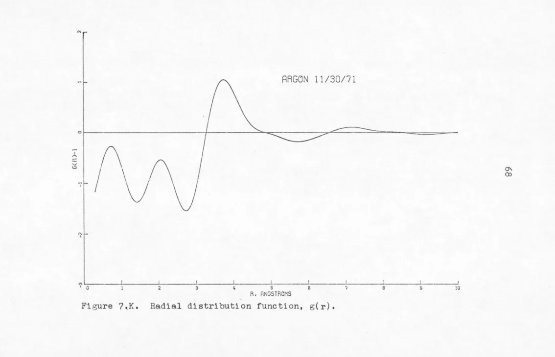
the decision is to be made relative to the existence of the peaks in i(s). In either Figure the third peak or valley is difficult to determine. There is a deviation from the gas scattering, but remember that this deviation must be multiplied by the independent variable in order to compute the Fourier transform.

Figures 7.A through 7,M and 8.A through 8.M present the various steps performed to obtain g(r), c(r) and the PY potential for the data of 11/J0/71 and 12/21/71. The structure factor, i(s), in each of these sets of Figures includes two positive peaks. This is to be contrasted in the numerical experiments with a parallel presentation of the 12/21/71 data with three peaks in i(s), hence the meaning of the

tl

on the 12/21/71 Figures.

Figures 7.A and 8.A each indicate the magnitude of the distortion correction relative to the uncorrected curve for the sample-detector distance used. This

(43)

the numerical experiments with the sample-detector dis-tance used by Mikolaj. 1

Figures 7.B and 8.B present the structure factor computed by Eq. (1). Note the isothermal compressibility effect on the 12/21/71 data as a decrease in i(O) relative to that of 11/J0/71.

In the following discussion of Figures 7. and 8. only the alphabetic identification will be referred to.

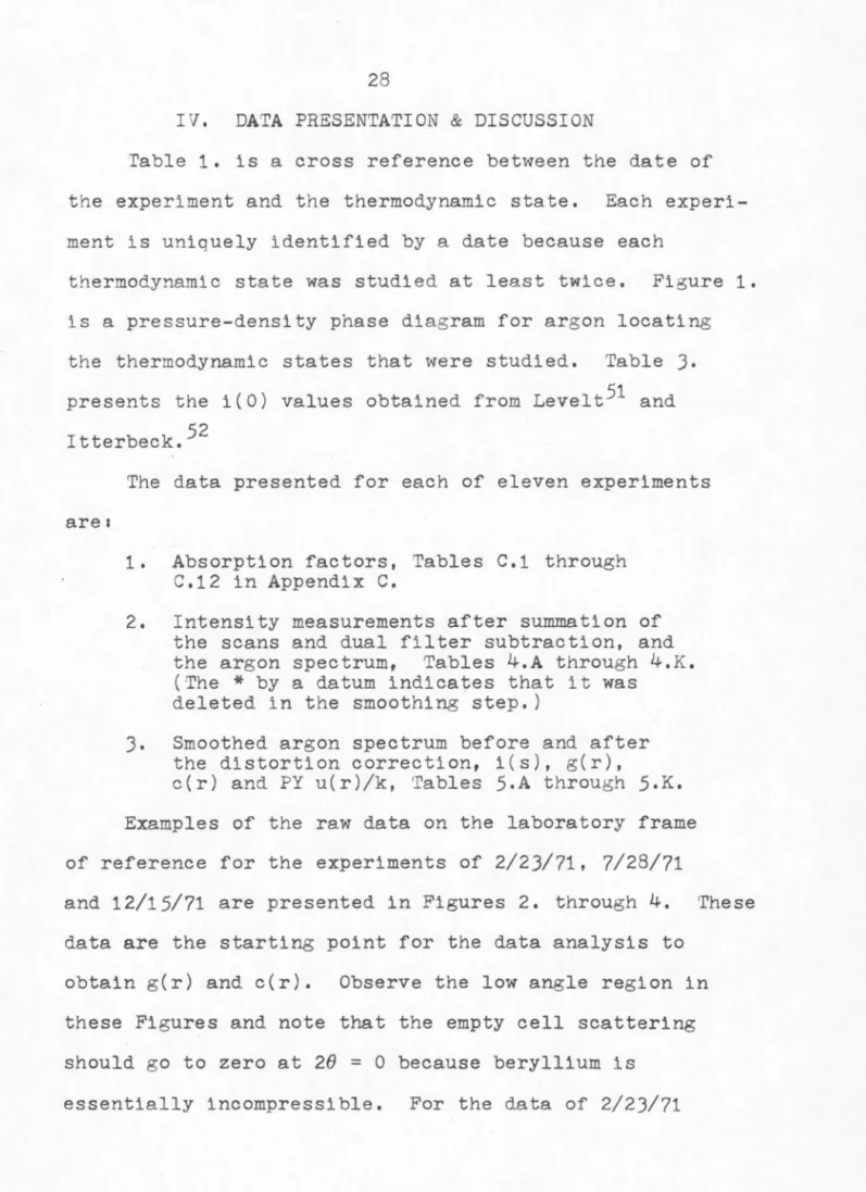
Figures C and D present the kernels of the Fourier

transforms of r[g(r)-1]

~nd

rc(r). The r[g(r)-1) kernels are rather uniform in appearance, but the rc(r) kernels

show a dominant feature in the region of 1

R-

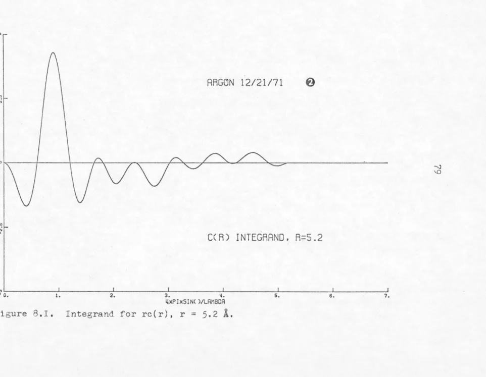
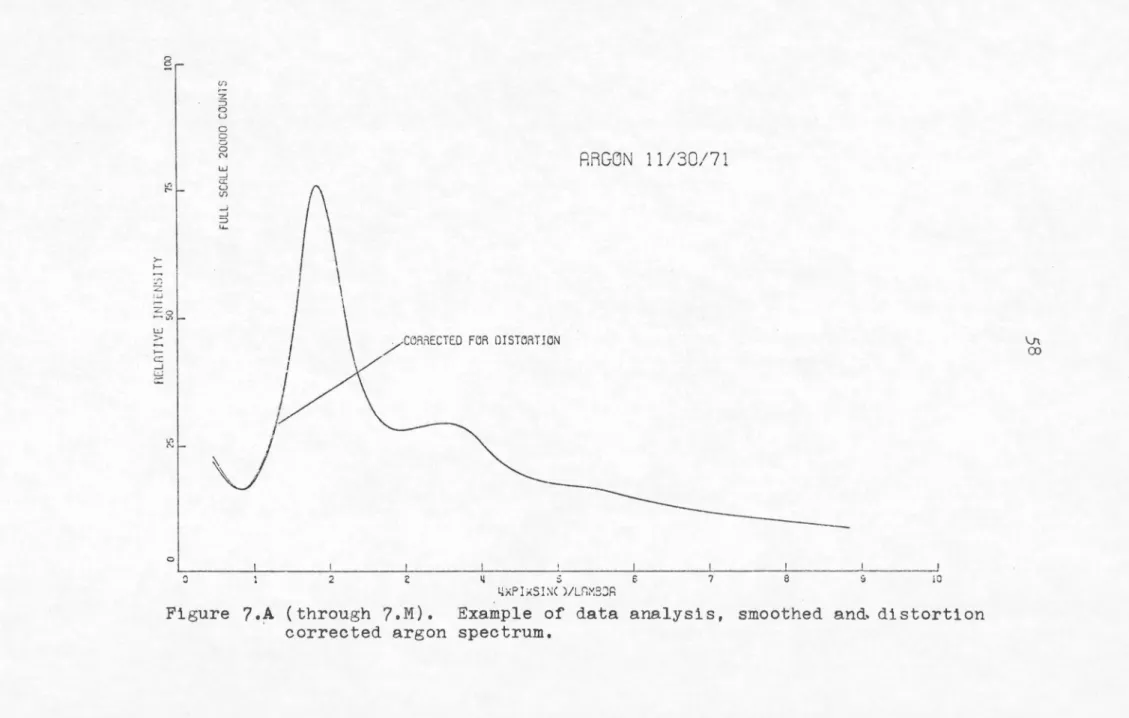
1• As the isothermal compressibility decreases, this feature becomes more pronounced.

Figures E through J present the actual curves to be integrated to obtain r(g(r)-1) and rc(r) for r

=

J.8, 5.2 and 7.2

i.

These quantities are then just the corre-sponding kernels multiplied by sin(sr). The area under the curve in the r

=

J.8

i

Figures is approximately g(r)-1 or c(r) since the lead constant on the integral,

(217"2pr)-1, is close to unity. The J.8

i

value of r is approximately where the maximum of g(r) and c(r) occur.

(44)

32

contributions to the integral are not small and to

compute g(r) or c(r) the difference of two relatively

large areas must be obtained and this is prone to

errors. Any error in determini ng i(s) in a small region

of s space, for example around 28

=

20, could easily 0

alter the result. This region of r space is where the

subsidiary peak appears in g(r) and a corresponding

second peak in c(r).

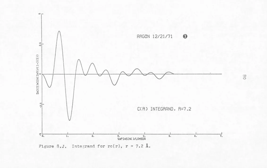
Figures G and J present the curves to be integrated

to obtai n r [g{r)-1] and rc(r) for r

=

7.2

R.

This is

the region in r space where the second peak in g{r)

appears. Note the dominant feature in the c(r) integrand

0-1. around 1 A

Figures K and L present the g(r)-1 and c(r)

esti-mates up to r

=

10

R.

The final Figures, M, present

the PY potentials for these two states.

A summary of the Percus-Yevick well depths, the

main peak height of i(s), g(r), c(r) and the width of

the main i(s) peak at i(s) = 0 is presented in Figures

(45)

V. NUMERICAL EXPERIMENTS

A. The Distortion Effect

It was previously noted in the Data Presentation

that the distortion correction applied to the data

in this work was relatively small. The reason for the

correction being small is that the sample-detector

dis-tance used was large relative to the sample length.

However, an interesting effect may be demonstrated if

a set of data. that has been corrected is numerically

distorted back to a smaller sample-detector distance,

thus mimicking the experimental conditions of Mikolaj,1

and then computing g(r), c(r) and the PY potential.

The distortion correction is described in Appendix G.

It is assumed that the sample-detector distance

used by Mikolaj was on the order of

4.8

inches.

Tables 7.A through 7.D present the results of

numerical experiments on the effect of distortion

car-ried out on four sets of reai data. These results

are to be compared with the corresponding correct data

in Tables 5.A through

5.K.

The result of computing g(r), c(r) and the PY

potential from data that appears as if they were obtained

with a sample-detector distance of

4.8

inches is a

marked decrease in the PY well depth. For the

(46)

34

on the order of 15°K. This error is also density

dependent as may be inferred from the derivation of

the correction procedure. The correction is slope

sensitive because the detector is an averager and

biased to high angles in the configuration used.

The numerical distortion experiment carried out

on the data of 6/23/71 is presented in plotted form

in Figures 14.A through 14.G. The most marked effect

is seen in Figure 14.D which shows the change in the

kernels of the Fourier transform of rc(r). It is true

that both g(r) and c(r) change in the same direction

upon correcting for distortion, but note that si(s)

is divided by l+i(s) to compute c(r), and in the region

of 1

i-

1, i(s) is less than zero, thus errors are

magnified and the change in c(r) is greater than in g(r).

Table 8. summarizes the results of the numerical

experiments on distortion relative to the PY well depths

for four experiments.

The distortion phenomenon explains why Mikolaj's

computed PY well depths are too small and the apparent

slope of these well depths verses density is too

steep.21,35

B. Subsidiary Peak Phenomenon

During the course of working up the data in this

thesis the so-called subsidiary peak2•4•40-44 sometimes

(47)

but an example of how i t may occur was obtained in the

data of 6/23/71 which are presented in Table

9.

The results for this set of data are plotted in

Figures 15.A through 15.E. On each of these Figures

there are two curves, one which yields the subsidiary

peak and one which does not. The decision to be made

is the choice between the two smoothed curves in Figure

15.A which represent the data on the laboratory frame

of reference.

It is interesting to note that there is a second

peak in c(r) when there ls a subsidiary peak in g(r)

for this set of data, hence, the local minimum on the

outer wall of the PY potential.

This demonstration does not present evidence either

pro or con relative to the existence of the subsidiary

peak. However, of all of the data presented in this

thesis, there are few occurrences of the subsidiary

peak and duplicate efforts did not yield the same

sub-sidiary peak. It may be said that the reproducibility

of the subsidiary peak at the present time is nonexistent.

c.

The Effect of Uncertainties in Smoothing Data in the Low Angle Region

During the course of examining the data from these

experiments, a few experimental measurements presented

PY well depths that were markedly too shallow or too deep.

(48)

36

known.

With

the aid of

duplicate

experiments on the

thermodynamic states studied,

it was guessed

that the

reason

had

something

to

do

with

the low angle region of

the data space.

Now a set of data

has

been prepared that shows the

sensitivity of c(r), but not

g(r), to the

smoothed line

estimate

in

the low

26 region.

The

data of 7/28/71

presented in Figures 16.A through 16.G show two parallel

work ups where everything is essentially the same except

that the first two data points in Figure 16.A are deleted

for one of the curves.

The reason for deleting data in this region is that

the detector had encountered the x-ray main beam.

Refer

back to Figure

3.

which is a plot of the raw data for

the experiment of 7/28/71 and note the increasing empty

cell intensity with decreasing angle.

Contrast this

observation against the raw data for the experiment of

2/23/71 which show the correct empty cell intensity

behavior.

The

important

Figure to observe in this sequence is

16.D which is a plot of the kernels of the Fourier

transform of rc(r).

The difference between the two

curves is relatively large around s

=

0.5

~-

1

,

and the

sine wave that multiplies these curves

for

the evaluation

(49)

c(r) plot and finally Figure

1

6.G which shows the

dif-ference

i

n the PY potentials.

The () and

t)

on these

Figures denote the same set of data in the sequence.

Qualitatively, c(r) increases as the smoothed line

estimate of the argon spectru

m

in the low s region is

biased upward.

The effect on g(r) for the same bias

of the smoothed line estimate is ni

l

.

Therefore, the

effect on the PY potential is a net decrease.

Table 10.A presents the data plotted in Figures

16.A through 16.G.

Table 10.B presents the data from

the experiment of

8/4/71

which yielded a PY well depth

that was too shallow as contrasted against the data of

the same experiment presented in Table 5.E.

The only

difference in these two sets of data again is the

low angle smoothed line estimate.

D.

Truncation, The Existence of a Third Peak in i(s)

at Various Pressures and the Effect of Neglecting It

The truncation of the structure factor, i(s), was

determined

bY

what could be observed from the raw data

on the laboratory frame of reference such as those

pre-sented in Figures 5. and

6.

To this date, argon spectra

such as these have never been presented in this form.

These spectra are the argon scatterin

g

as observed by the

detector.

No corrections have been made and only the

cell scattering has been subtracted off.

(50)

38

4~

K-l

are on the order of the scatter of the data.

To be emphasized is the fact that in the ensuing data analysis the gas scattering is subtracted from the data and the result multiplied by the independent variable, thus errors are also multiplied.

The structure factor is state dependent. For two

thermodynamic states on an isotherm, i(s) for the higher pressure state is expected to have larger peak heights due to an increase in packing over the lower pressure state.

0

Three thermodynamic states on the 127 K isotherm

were studied. The pressures of these states were

54.4,

36.8

and 18.7 atm. Therefore, these data can be used

to infer information about the observability of the third peak in i(s) and the effect of truncating it.

The experiment of 12/15/71 was conducted at 54.4

0

atm and 127 K and the argon spectrum is presented in Figure

6.

This Figure indicates that there might

possibly be an observable third peak in i{s). There-fore, to determine the effect of neglecting the third peak, or truncating it, these data were worked up with and without it.

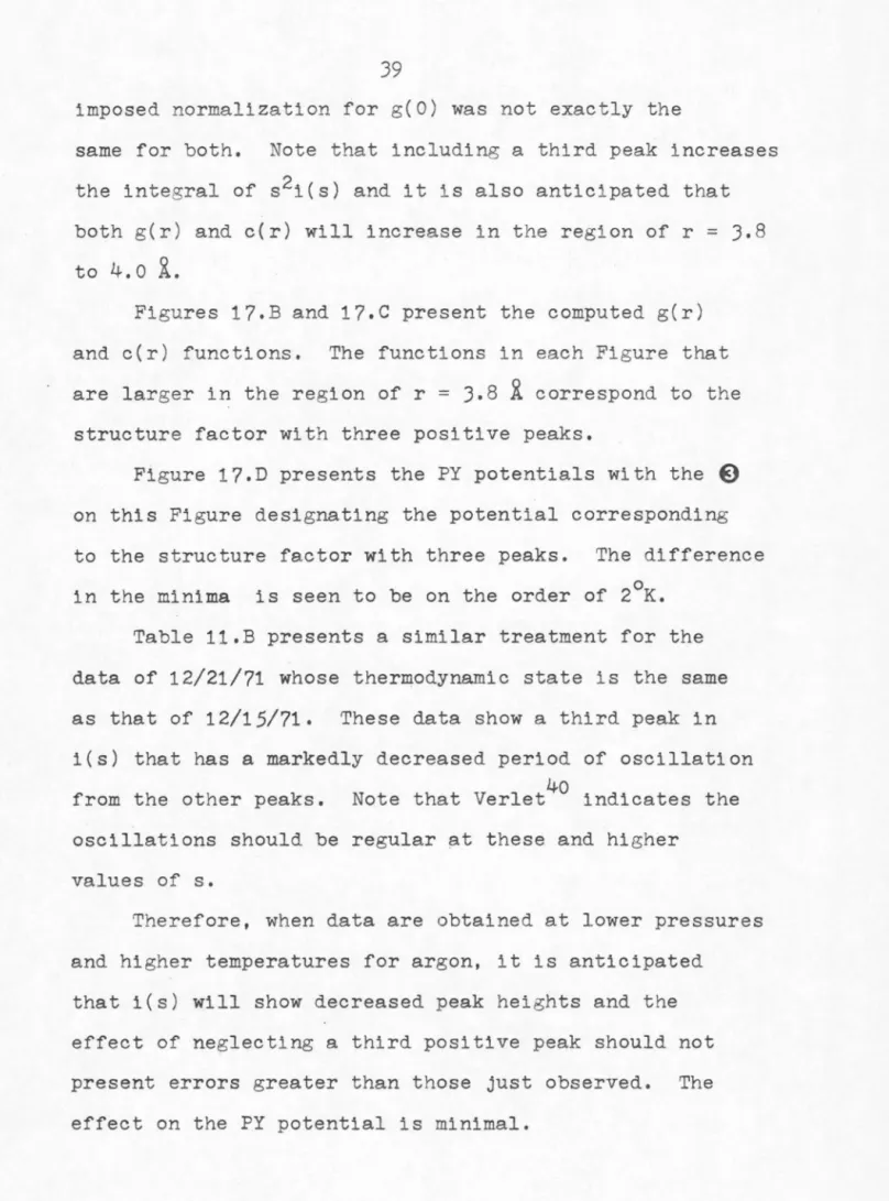
Figures 17.A through 17.D and Table 11.A present i(s), g(r), c(r) and the PY potential for this case. The structure factors in Figure 17.A show a slight

(51)

imposed normalization for g(O) was not exactly the

same for both. Note that including a third peak increases

the integral of s 2i(s) and i t is also anticipated that both g(r) and c(r) will increase in the region of r

=

3.8

to

4.o

R.

Figures

17.B

and

17.c

present the computed g(r)

and c(r) functions. The functions in each Figure that are larger in the region of r

=

3.8

R

correspond to the structure factor with three positive peaks.

Figure

17.D

presents the PY potentials with the €)

on this Figure designating the potential corresponding

to the structure factor with three peaks. The difference in the minima is seen to be on the order of 2°K.

Table

11.B

presents a similar treatment for the

data of

12/21/71

whose thermodynamic state is the same as that of

12/15/71.

These data show a third peak in

i(s) that has a markedly decreased period of oscillation

40

from the other peaks. Note that Verlet indicates the oscillations should be regular at these and higher

values of s.

Therefore, when data are obtained at lower pressures and higher temperatures for argon, i t is anticipated

that i(s) will show decreased peak heights and the effect of neglecting a third positive peak should not present errors greater than those just observed. The

(52)

40

E. Effect of g{O) Being Significantly Different from Zero

In the Data Analysis Section i t was stated that

the computed g(O) value was being used as a guide to

yield information about the normalization of i(s). To

determine the effect of the choice of the normalization

criterion used, a study was carried out allowing g(O)

to assume positive values significantly different from

zero to observe the effect on g(r), c(r) and the PY

potential.

The data of 11/30/71, which include in the structure

factor two positive peaks, were reworked and the g(O)

value forced positive by truncating i(s) at a different

value of s. Figures 18.A through 18.D and Tables 12.A

through 12.B present two parallel work ups for i(s)

which give g(O) values of about +3 and +6. Note

in these Figures that the effect on g(r) at r

=

3,8 ~

is somewhat less than on c(r). The PY well depth for

the +3 case is about 114°K and for the +6 case about

109°K.

Also note that in forcing g(O) positive that the

third valley i~ i(s) almost disappeared. 'rhis is in

40

contrast to the behavior expected by Verlet.

Compare these well depths to the 11/30/71 data in

Table 5.H where the well depth is 120°K for g(O) ~ -0.5.

(53)

Actually, the value of g(O) cannot be discussed

without taking into account truncation. If a t hird peak

had been i ncluded in the set of data used in this

numer-ical experiment, g(O) would have been larger.

Therefore, to estimate an upper bound on the

contri-bution to g(O) from a neglected third peak in i(s),

consider the following. The third vall ey of i(s) in

the 11/30/71 data in Table 5.H was multiplied by -1 and

shifted up i n s space by 1.12

R-l

to mimic a third

peak. Integrating s 2 i(s) over this assumed third peak

2

-1

and multiplying by (277'

p)

yielded about

4.5.

Using

this as an extreme upper bound, g(O) would be expected

to be about

-J.5

neglecting the third peak in i(s).

Note that the amplitude of each successive

oscil-lation of i(s) appears to decrease by about a factor of

two, and also in this particular case the third valley

appears to span too great a range in s space. Therefore,

to be more realistic, neglecting the third peak should

yield g(O) on the order of -2.

This experimental evidence indicates that positive

g(O) values are not plausible when a third peak in

i(s) is neglected. Also, if three peaks and valleys

are included, i t is plausible to expect g(O) to be

close to zero. Peaks higher in s space are not expected

(54)

42

Therefore, if argon data for the states studied are

presented that yield positive g(O) values significantly

different from zero, for example +10, then the PY well

depth will be shallow by approximately 15°K. If a

third peak is included in i(s), then there will be three

negative and three positive peaks and the computed g(O)

value should be quite close to zero. The assumed negative

bias of g(O) in this work appears to be reasonable.

F. Effect on g(r) and c(r) Using Post- vs. Pre-cell Alignment for Computing Absorption Factors

In the Data Analysis i t was stated that the cell

moved during the course of an experiment. The cell

position in the x-ray main beam must be known to

com-pute absorption factors. In order to evaluate the

effect of such movement on final results, the data of

9/28/71 were worked up with both sets of absorption

factors. The post-alignment was approximately 0.001

inch lower.

The changes in g(r) and c(r) were not large, g(r)

being either 2.09 or 2.06 at J.8 ~. and c(r) being either

1.21 or 1.18 at 3,9

~.

The PY well depth changed by

approximately

2°K

at 4.0 ~. Table lJ. presents the data

worked up with the post-alignment absorption factors

designated as (II) and Table

5.G

presents the

pre-alignment case designated as (I). The absorption factors

(55)

Therefore, cell movement during an experiment did

(56)

44

VI.

CONCLUSIONS AND

RECOMMENDATIONS

A summary of the PY well depths, main peak heights of i(s), g(r) and c(r) is presented in Figures

9,

through 12. These Figures give an estimate of the experimental reproducibility. These results are best estimates based on the numerical experiments presented. There is no reason to believe that the scatter in the final results

is due to any cause other than the scatter in the data on the laboratory frame of reference.

The following question arises. Will the results

0

change appreciably, for example, ±10 K on the PY well depths, if better .experimental or numerical techniques were developed and used? The answer, though somewhat subjective, is no for the following reasons.

The divergence correction relies on the stated

assumption of a nondivergent, or perfect, main beam. It is estimated that a change of not more than a

S°K

increase

in the well depth would occur if the main beam divergence was considered, This estimate is based on the fact that the x-ray target to sample distance is greater than the sample to detector distance and in the configuration used,

an error of

S°K

would have occurred if the data were not corrected for the sample to detector distance. Also the main beam was collimated.

(57)

factors used are based on a free atom and do not take into account the fact that neighbors are present. The effect of this approximation on the results is not

obvious, but a significant effect is not expected. The lack of data in the low s region and the need

for interpolation to s

=

O possibly results in an error in c(r). Numerical experiments on this aspect suggest

0

that an error of 10 K in the computed well depths is possible, but the sign of this error is not evident.

This problem is definitely important because of the compressibility of argon for the thermodynamic state·s studied, and hence, the effect on the kernel of the

Fourier transform of rc(r).

The effect of double scattering5J,S

4

was not

con-sidered. This phenomenon arises from the fact that a photon may actually be scattered twice rather than once

before entering the detector. The possible paths then

could be cell to cell, sample to sample, cell to sample and sample to cell. The effect of this phenomenon on the final results was not investigated, but a significant effect is not expected.

At this point, i t is anticipated that there is no

other important experimental phenomenon that has not been considered or mentioned.

(58)

46

this thesis, the following conclusions relative to

current statistical mechanical theories of fluids may

be drawn:

1. The Percus-Yevick well depths, u(r)/k, for argon

computed from measured g(r) and c(r) functions are in

0

the range of 105 to 120 K for the five states of argon

studied. Because of the narrow density range studied,