University of Huddersfield Repository
Malviya, Vihar, Mishra, Rakesh, Palmer, Edward and Majumdar, Bireswar
CFD Based Analysis of the Effect of MultiHole Pressure Probe Geometry on Flow Field
Interference
Original Citation
Malviya, Vihar, Mishra, Rakesh, Palmer, Edward and Majumdar, Bireswar (2007) CFD Based
Analysis of the Effect of MultiHole Pressure Probe Geometry on Flow Field Interference. In: Fluid
mechanics and Fluid Power. Birla Institute of Technology, pp. 113122.
This version is available at http://eprints.hud.ac.uk/id/eprint/6132/
The University Repository is a digital collection of the research output of the
University, available on Open Access. Copyright and Moral Rights for the items
on this site are retained by the individual author and/or other copyright owners.
Users may access full items free of charge; copies of full text items generally
can be reproduced, displayed or performed and given to third parties in any
format or medium for personal research or study, educational or notforprofit
purposes without prior permission or charge, provided:
•
The authors, title and full bibliographic details is credited in any copy;
•
A hyperlink and/or URL is included for the original metadata page; and
•
The content is not changed in any way.
For more information, including our policy and submission procedure, please
contact the Repository Team at: [email protected].
CFD BASED ANALYSIS OF THE EFFECT OF MULTI-HOLE
PRESSURE PROBE GEOMETRY ON FLOW FIELD
INTERFERENCE
V Malviya
a, R Mishra
a, E Palmer
a, B Majumdar
ba
University of Huddersfield, Queensgate, Huddersfield, HD1 3DH, U.K.
bJadavpur University, Salt Lake Campus, Salt Lake City , Block-LB, Plot No. 8,
Sector –III, Calcutta, 700091, India.
Abstract
Multi-hole pressure probes are extensively used to characterise three dimensional flows in difficult applications [1,2]. These probes provide sufficiently accurate information about flow velocity. They have the advantages of being, usable with high temperature fluids, simple to fit have practically no additional flow losses
In this paper the influence of the probe geometry on the flow field disruption has been reported. The values and ranges of variations of the flow field parameters in the model have been assessed on the basis of the numerically computed velocity and pressure fields around and inside the probe [3]. For this probe interior details have been modelled fairly accurately.
The flow field has been predicted using computational fluid dynamics and the characteristics linking the degree of interference with probe head shape have been presented. The conclusions have been formulated taking complex flow metrology needs into account.
1
Nomenclature
Re = Reynolds number
ρ = density
k = turbulence kinetic energy ε = turbulence dissipation rate
PCENTRE = Pressure at centre hole
PLEFT = Pressure at left hole
PRIGHT = Pressure at right hole
PTOP = Pressure at top hole
PBOTTOM = Pressure at bottom hole
PAVG = Average of peripheral pressures
4 P P P P
P LEFT RIGHT TOP BOTTOM AVG
CPITCH = coefficient of pitch
CYAW = coefficient of yaw
QP = coefficient of dynamic pressure
SP = coefficient of total pressure
2
Introduction
optimised head geometry for efficient application of these instruments.
Pressure probe optimisation is an arduous process, as it involves repetitive designing and testing of several geometric parameters such as probe head diameter, head shape, shaft size, shaft shape and the distance between the probe head and the probe shaft. This process can be simplified by numerically analysing of the flow field in and around such probes which can assist in their efficient design. The resulting geometric modifications can contribute to significant reduction in flow field interference caused by the probes. This will consequently minimise the errors caused due to interaction of adjacent probes. However little or no work has been reported on the numerical optimisation of the geometry of such probes.
Although advanced machining resources are now available, reducing the size of probe head is not the direct solution for optimising probe design. Decreasing the probe head diameter past 0.2mm yields unacceptable response times of the pressure taps [4], thus inhibiting their use in unsteady applications.
While minimising the interference due to pressure probes is important, calibration of these pressure probes for the required range of measurement is also very important for accurate flow mapping applications. Due to the practical limitations in machining techniques and maintaining consistent standard calibration conditions, full three dimensional calibration as discussed by Bryer and Pankhurst [1] and Morrison et al [2] are becoming common practice. These techniques establish a relationship between the five pressure outputs of the probe and the velocity vector of air under standard conditions. As discussed by Coldrick, et al. [5], a unique dimensionless coefficient is required for each quantity to be measured. This coefficient needs to be dominantly influenced by the corresponding quantity and less influenced by other quantities. These coefficients are given by Bryer and Pankhurst [1] as:
AVG CENTRE
TOP BOTTOM P ITCH
P P
P P
C
1
AVG CENTRE
LEFT RIGHT
YAW P P
P P C
2
STATIC TOTAL
AVG CENTRE
P P P
P P
Q
3
AVG CENTRE
CENTRE TOTAL
P P P
P P
S
4
CPITCH is more sensitive to variation in pitch
than other parameters; CYAW on the other hand, is more sensitive to variations in yaw than other parameters. Similarly, QP and SP are both more sensitive to variation in velocity and represent changes in total and static pressures. The calibration surfaces corresponding to the four calibration coefficients in combination with known pitch and yaw are utilised to develop a parametric relationship between the pressures at the five pressure taps of the probe and the magnitude and direction of the velocity of air with respect to the probe head axis [1].
It is imperative that the probe head is designed in such a way that the pressures at the five taps represent the velocity vector. In order to achieve this left and right taps should be chiefly sensitive to variation in yaw and the top and bottom taps to pitch. However this is not the case in practice and several other factors like tap location and shaft interference [4] influence the characteristic responses of the pressure taps, thus producing inaccurate calibration coefficients.
The contours of the calibration surface also indicate the measurable ranges of flow angles and also anomalies in probe head manufacture, if any [2].
problem cannot be resolved by including standard correction factors for inter-probe interaction in the calibration process. Optimum probe design will not only reduce such interference but also result in increased accuracy of the calibration coefficients. Various probe head geometries have been discussed by Bryer and Pankhurst [1] however; a detailed comparative analysis of these head shapes is required to understand the relationship between geometric parameters and their influence on flow field interference.
This paper presents an analysis of the interference caused by conical and hemispherical head probes by studying the variation of static pressure, vertical (Y) and lateral (Z) components of velocity and presents a comparison between these head geometries. This work proposes to provide essential information regarding placement of multiple pneumatic probes for a novel wheel arch flow mapping study. This work uses computational techniques to employ numerical simulation of the flow in and around the probe heads. The analysis is aimed at generating detailed information regarding the flow around the probe head. This information will help with relating flow field characteristics to probe geometry so that future probe designs cause minimal interference and provide suitable accuracy.
3
Computational Details
The flow field around the probe and in the tubes is simulated mathematically using computational fluid dynamics (CFD). This includes a set of partial differential equations and boundary conditions. The CFD package
Fluent 6.0 [7] is used to iteratively solve
Navier-stokes equations along with the continuity equations and appropriate auxiliary equations depending on the type of applications using a control volume formulation. In this study the conservation equations for mass and momentum have been solved sequentially with two additional transport equations for steady turbulent flow. Linearisation of the governing equations is implicit.
3.1 Mass Conservation
The mass conservation equation given below is valid for both incompressible and compressible flows. The source term Sm is the mass added to the continuous phase from the dispersed second phase (e.g. Due to vaporization of liquid droplets) and any user defined sources [7].
m
S
v
t
(
)
5 [7]
3.2 Momentum Conservation
Conservation of momentum in the ith direction in an inertial (non accelerating) reference frame is given by
F g p
v v t
u
) ( )
( ) (
6 [7]
The stress tensor is given by
]
3
2
)
[(
v
v
Tv
I
ij
7 [7]
Where μ is the molecular viscosity, I is the unit tensor, and the second term on the right hand side is the effect of volume dilation.
Fluent uses the finite volume method to solve
integration, is the step that distinguishes the finite volume method from other CFD methods. The statements resulting from this step express the conservation of the relevant properties for each finite cell volume [8].
3.3 Boundary Conditions
Each computational simulation employed a three dimensional model of the five-hole pressure probe of 5mm outer diameter and 1mm internal pressure taps. The probe was modelled in a computational domain of identical geometry to the wind tunnel test section at the University of Huddersfield. The test section consists of 230 x 230 mm cross section. The computational domain was discretised by the pre-processor GAMBIT [6], as shown in Figure 1b. By employing an unstructured meshing scheme a fine mesh was generated near the probe and a coarse mesh near the domain extremities. A mesh optimisation analysis yielded a discretised solution domain with approximately 1.8 million tetrahedral elements.
Boundary conditions were formulated to accurately represent the experimental wind tunnel study. Using boundary conditions that accurately represent actual experimental calibration process is fundamental if the results are expected to be meaningful. The pneumatic probes were each modelled to be stationary in air travelling at a constant velocity of 33.7m/s. The outlet boundary was implemented to be at an atmospheric pressure of 101325 Pa. The walls of the probes and the solution domain are represented as smooth zero shear slip walls. In the present analysis flow is assumed to be turbulent as the Reynolds numbers of the flow is 1.08 × 10⁴ over the pneumatic probe. To model the turbulence the semi-empirical k-ε turbulence RNG model is employed in this study as it was found to give stronger convergence than the standard k-ε model. A complete summary of the boundary conditions used is given in Figure 3.
The solution was obtained on a workstation with an Intel Core 2 Duo® (E6300) processor and 4 gigabyte of system memory, using a
steady state solution scheme in a run time of approximately 6 hours for each run.
3.4 Parameters
Three dimensional models of both a conical and hemispherical headed probe have been analysed (as shown in Figure 2a) and Figure 2b respectively). Each probe was simulated at 0º yaw and 0º pitch.
4
Results and Discussion
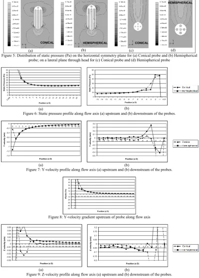
4.1 Pressure Distribution in Flow Field Static pressure in the flow field around the probe is a direct indication of how the probe influences the flow field. Figure 5 shows distribution of static pressure around the heads of the conical and hemispherical probes at 0º yaw. Just as theoretically expected and also discussed by Morrison et al. [2], the distribution of pressure around the probe is reasonably symmetric as the probe head axis is oriented into the flow at 0º yaw and 0º pitch. This distribution profile also indicates that the static pressure distribution in the flow field around both probes is largely similar.
4.2 Pressure Distribution along Flow Axis
For comparing the effect of the probe on the flow field around it, static pressure values along the flow axis upstream as well as downstream are plotted in Figure 6a and Figure 6b respectively.
A comparison of these static pressure values for both head shapes indicates that the hemispherical head shape causes lesser disruption of flow field; this is because for upstream values (Figure 6a) although the gradient is similar, the pressure rises about 0.5D later for the hemispherical head shape than for the conical head shape. In case of downstream values (Figure 5b) the static pressure value for the hemispherical head probe drops to about 15Pa at a distance of 3D downstream whereas for the conical head probe, the static pressure drops to about 15Pa at a distance of 5D downstream. This clearly indicates that the influence of the probe on the flow field is greater for the conical head shape than the hemispherical.
4.3 Velocity Distribution along Flow Axis
The transverse components of velocity in the vertical (Y) and lateral (Z) directions give a reasonable indication of the disruption of the flow field caused by the probe. It clearly follows that the influence of the probe decreases as these components fall to near-zero values and the magnitude of velocity is dominated by the longitudinal (X)
component. A comparison of Y-velocity and Z-velocity along the flow axis is plotted in Figure 7 and Figure 9.
Figure 7a shows the distribution of the Y- velocity along the flow axis upstream of the probe. Although the hemispherical head shows a higher negative value of Y-velocity then the conical head immediately upstream of the probe, it reduces sharply as we move away from the probe in the upstream direction. This can be clarified by the gradient of Y-velocity with respect to positions along the x-axis illustrated in Figure 8; here it is clear the Y-velocity for the hemispherical head falls sharply at 2D, whereas that for the conical head decreases gradually as we move away from the probe upstream. Figure 7b shows the Y-velocity distribution along the flow axis downstream of the probes. It is clear from this plot that the Y-velocity for the hemispherical head shape reaches near-zero value at a distance of approximately 9D downstream, whereas for the conical head shape the Y-velocity maintains about -0.05m/s even beyond 15D. This clearly indicates that the conical head shape influences the flow field far beyond the influence of the hemispherical shape downstream.
5
Conclusions
The flow field around conical head and hemispherical head pneumatic probes has been studied using CFD techniques. The static pressure distribution around the probes for both head shapes has been presented with transverse velocity profiles along the flow axis upstream and downstream of the probes. Although the influence of both head shapes on static pressure and transverse velocity components are similar upstream of the probes, the extent of disruption caused downstream is significantly diverse. Up to a distance of two head diameters downstream of the probe the conical head is seen to have a much larger disruptive influence on the flow field. This is shown by the higher values of static pressure for the conical head within this region indicating a higher level of flow divergence. The average static pressure between one and five diameters downstream of the probe is 7.8% higher for the conical head compared to the hemispherical probe. This is supported by the generally higher values of Y and Z components of velocity for the conical head. The Y-velocity for the hemispherical head shape observed at 10D downstream is more than 90% lower, at 0.0025m/s, than the conical head shape.
The influence of the hemispherical head probe on the flow beyond 6D upstream and 10D downstream is minimal. At these distances from the probe the effect on the flow is considered to be marginal; the transverse velocity components have become less than 0.5% of the free stream velocity upstream and less than 0.2% downstream.
Although these influences can be further reduced by reducing the size of the probes the conical probe will always have a larger effect on the flow field for similar sized probe heads. The lower effect of the hemispherical probe on the measured flow will subsequently improve the accuracy of the measurements. Also due to the lower level of flow disruption caused by the hemispherical head it is possible to use a denser distribution of probes of this type compared to the conical
head. Therefore it can be concluded that the hemispherical head shape is advantageous over the conical probe in complex flow mapping applications where multiple pneumatic probes may be used.
6
References
1. Bryer, D.W. and Pankhurst, R.C. (1971). Pressure-probe methods for determining
wind speed and flow direction. London
(UK): Her Majesty’s Stationary Office. 2. Morrison, G.L., Schobeiri, M.T. and
Pappu, K.R. (1998). ‘Five-hole pressure probe analysis technique’. Flow
Measurement and Instrumentation.
Volume 9, Part 3: pp. 153-158. 3. Dobrowolski, B., Kabacinski, M. and
Pospolita, J. (2005). ‘A mathematical model of the self-averaging Pitot tube. A mathematical model of a flow sensor’.
Flow Measurement and Instrumentation.
Volume 16: pp 251-265.
4. Depolt, Th. and Koschel, W. (1991). ‘Investigation on Optimizing the Design Proces of Multi-Hole Pressure Probes for Transonic Flow with Panel Methods’. In: IEEE, ICIASF '91 Record,International Congress on Instrumentation in
Aerospace Simulation Facilities, New
York (USA), pp. 1-9. IEEE.
5. Coldrick, S., Ivey, P. and Well, R. (2003). ‘considerations for Using 3-D Pneumatic Probes in High-Speed Axial Compressors’. Journal of
Turbomachinery. Volume 125, Part 1:
pp. 149-154.
6. Fluent, Inc. Gambit 2.0.4 (Geometry and mesh generation pre-processor for Fluent).
7. Fluent, Inc. Fluent 6.0.12 (flow modelling software).
8. Palmer, E., Mishra, R. and Fieldhouse, J. (2007) ‘The Manipulation of Heat Transfer Characteristics of a Pin Vented Brake Rotor Through the Design of Rotor Geometry’ (AE14-3). In: EAEC,
11th European Automotive Congress,
May 30 – 1 June, 2007, Budapest
Figures
(a) (b)
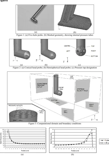
Figure 1: (a) Five-hole probe. (b) Meshed geometry, showing internal pressure tubes
(a) (b) (c)
Figure 2: (a) Conical head probe; (b) Hemispherical head probe; (c) Pressure tap designation
Figure 3: Computational domain and boundary conditions
0 10 20 30 40 50 60 70 80 90 100
0 1 2 3 4 5 6 7 8 9 10 11 12 13 14 15 16 17 18 19 20
Position (x D)
S
ta
ti
c
P
re
s
s
u
re
(
P
a
)
(a)
0 10 20 30 40 50 60
-15 -14 -13 -12 -11 -10 -9 -8 -7 -6 -5 -4 -3 -2 -1 -0
Position (x D)
S
ta
ti
c
P
re
s
s
u
re
(
P
a
)
[image:8.595.104.489.128.675.2](b)
(a) (b) (c) (d)
Figure 5: Distribution of static pressure (Pa) on the horizontal symmetry plane for (a) Conical probe and (b) Hemispherical probe; on a lateral plane through head for (c) Conical probe and (d) Hemispherical probe
0 5 10 15 20 25 30 35 40 45 50 0.00
6 1 2 3 4 5 6 7 8 9 10 11 12 13 14 15 16 17 18 19 20
Position (x D)
S ta ti c P re s s u re ( P a ) (a) 0 10 20 30 40 50 60
-15 -14 -13 -12 -11 -10 -9 -8 -7 -6 -5 -4 -3 -2 -1 -0.01
Position (x D)
S ta tic P re ss u re (P a) (b)
Figure 6: Static pressure profile along flow axis (a) upstream and (b) downstream of the probes.
-1.4 -1.2 -1 -0.8 -0.6 -0.4 -0.2 0
0 1 2 3 4 5 6 7 8 9 10 11 12 13 14 15 16 17 18 19 20
Position (x D)
Y v e lo c it y ( m /s ) (a) -0.5 -0.4 -0.3 -0.2 -0.1 0 0.1 0.2 0.3 0.4
-15 -14 -13 -12 -11 -10 -9 -8 -7 -6 -5 -4 -3 -2 -1 -0
Position (x D)
Y v e lo c it y ( m /s ) (b)
Figure 7: Y-velocity profile along flow axis (a) upstream and (b) downstream of the probes.
-50 -40 -30 -20 -10 0 10 20 30 40 50
0 1 2 3 4 5 6 7 8 9 10 11 12 13 14 15 16 17 18 19 20
Position (x D)
d V y/ d x (1 /s )
Figure 8: Y-velocity gradient upstream of probe along flow axis
-0.05 -0.04 -0.03 -0.02 -0.01 0 0.01 0.02 0.03 0.04 0.05
0 1 2 3 4 5 6 7 8 9 10 11 12 13 14 15 16 17 18 19 20
Position (x D)
Z v el o ci ty ( m /s ) (a) -0.2 -0.15 -0.1 -0.05 0 0.05 0.1 0.15 0.2
-15 -14 -13 -12 -11 -10 -9 -8 -7 -6 -5 -4 -3 -2 -1 -0
Position (x D)
[image:9.595.98.498.124.684.2]Z v e lo c it y ( m /s ) (b)
Figure 9: Z-velocity profile along flow axis (a) upstream and (b) downstream of the probes.